1. Introduction to CNN

1. Neural Network Basics

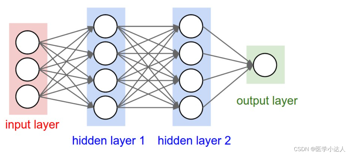
In the input layer (Input layer), many neurons (Neuron) receive a large amount of nonlinear input information. The input information is called the input vector.
Output layer (Output layer), the information is transmitted, analyzed, and weighed in the neuron link to form the output result. The output message is called the output vector.
Hidden layer , referred to as "hidden layer", is a layer composed of many neurons and links between the input layer and the output layer. If there are multiple hidden layers, that means multiple activation functions.

2. Convolve it

The Convolutional Neural Network ( CNN ) has amended the limitations of the fully connected network by adding a convolutional layer (Convolution layer) and a pooling layer (Pooling layer). Usually, a convolutional neural network consists of several convolutional layers (Convolutional Layer), activation layer (Activation Layer), pooling layer (Pooling Layer) and fully connected layer (Fully Connected Layer).

Let's see how to convolute

1. As shown in the figure, you can see:

（1）两个神经元，即depth=2，意味着有两个滤波器。
（2）数据窗口每次移动两个步长取3*3的局部数据，即stride=2。
（3）边缘填充，zero-padding=1，主要为了防止遗漏边缘的像素信息。
    然后分别以两个滤波器filter为轴滑动数组进行卷积计算，得到两组不同的结果。

2.如果初看上图，可能不一定能立马理解啥意思，但结合上文的内容后，理解这个动图已经不是很困难的事情：

（1）左边是输入（7*7*3中，7*7代表图像的像素/长宽，3代表R、G、B 三个颜色通道）
（2）中间部分是两个不同的滤波器Filter w0、Filter w1
（3）最右边则是两个不同的输出
（4）随着左边数据窗口的平移滑动，滤波器Filter w0 / Filter w1对不同的局部数据进行卷积计算。

局部感知：左边数据在变化，每次滤波器都是针对某一局部的数据窗口进行卷积，这就是所谓的CNN中的局部感知机制。打个比方，滤波器就像一双眼睛，人类视角有限，一眼望去，只能看到这世界的局部。如果一眼就看到全世界，你会累死，而且一下子接受全世界所有信息，你大脑接收不过来。当然，即便是看局部，针对局部里的信息人类双眼也是有偏重、偏好的。比如看美女，对脸、胸、腿是重点关注，所以这3个输入的权重相对较大。
参数共享：数据窗口滑动，导致输入在变化，但中间滤波器Filter w0的权重（即每个神经元连接数据窗口的权重）是固定不变的，这个权重不变即所谓的CNN中的参数（权重）共享机制。

3卷积计算：

图中最左边的三个输入矩阵就是我们的相当于输入d=3时有三个通道图，每个通道图都有一个属于自己通道的卷积核，我们可以看到输出（output）的只有两个特征图意味着我们设置的输出的d=2，有几个输出通道就有几层卷积核（比如图中就有FilterW0和FilterW1），这意味着我们的卷积核数量就是输入d的个数乘以输出d的个数（图中就是2*3=6个），其中每一层通道图的计算与上文中提到的一层计算相同，再把每一个通道输出的输出再加起来就是绿色的输出数字啦！
举例：

绿色输出的第一个特征图的第一个值：

1通道x[ : :0] 1*1+1*0 = 1 （0像素点省略）

2通道x[ : :1] 1*0+1*(-1)+2*0 = -1

3通道x[ : :2] 2*0 = 0 

b = 1

输出：1+（-1）+ 0 + 1（这个是b）= 1 

绿色输出的第二个特征图的第一个值：

1通道x[ : :0] 1*0+1*0 = 0 （0像素点省略）

2通道x[ : :1] 1*0+1*(-1)+2*0 = -1

3通道x[ : :2] 2*0 = 0 

b = 0

输出：0+（-1）+ 0 + 1（这个是b）= 0

二、CNN实例代码：

import torch
import torch.nn as nn
from torch.autograd import Variable
import torch.utils.data as Data
import torchvision
import matplotlib.pyplot as plt

模型训练超参数设置，构建训练数据：如果你没有源数据，那么DOWNLOAD_MNIST=True

#Hyper prameters
EPOCH = 2
BATCH_SIZE = 50
LR = 0.001
DOWNLOAD_MNIST = True
 
train_data = torchvision.datasets.MNIST(
    root ='./mnist',
    train = True,
    download = DOWNLOAD_MNIST
)

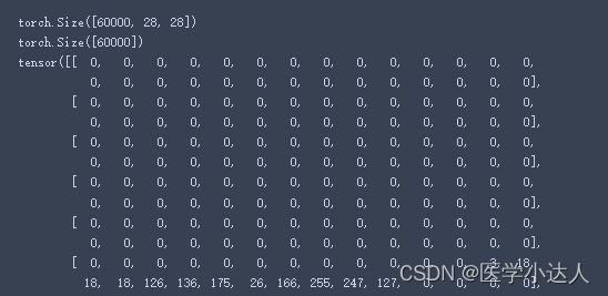
数据下载后是不可以直接看的，查看第一张图片数据：

print(train_data.data.size())
print(train_data.targets.size())
print(train_data.data[0])

结果：60000张图片数据，维度都是28*28，单通道

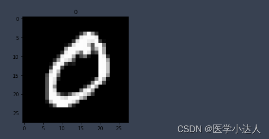
画一个图片显示出来

# 画一个图片显示出来
plt.imshow(train_data.data[0].numpy(),cmap='gray')
plt.title('%i'%train_data.targets[0])
plt.show()

结果：

训练和测试数据准备，数据导入：

#训练和测试数据准备
train_loader=Data.DataLoader(dataset=train_data, batch_size=BATCH_SIZE, shuffle=True)
 
 
test_data=torchvision.datasets.MNIST(
    root='./mnist',
    train=False,
)
 
#这里只取前3千个数据吧，差不多已经够用了，然后将其归一化。
with torch.no_grad():
    test_x=Variable(torch.unsqueeze(test_data.data, dim=1)).type(torch.FloatTensor)[:3000]/255   
    test_y=test_data.targets[:3000]

注意：这里的归一化在此模型中区别不大

构建CNN模型:

'''开始建立CNN网络'''
class CNN(nn.Module):
    def __init__(self):
        super(CNN,self).__init__()
        '''
        一般来说，卷积网络包括以下内容：
        1.卷积层
        2.神经网络
        3.池化层
        '''
        self.conv1=nn.Sequential(
            nn.Conv2d(              #--> (1,28,28)
                in_channels=1,      #传入的图片是几层的，灰色为1层，RGB为三层
                out_channels=16,    #输出的图片是几层
                kernel_size=5,      #代表扫描的区域点为5*5
                stride=1,           #就是每隔多少步跳一下
                padding=2,          #边框补全，其计算公式=（kernel_size-1）/2=(5-1)/2=2
            ),    # 2d代表二维卷积           --> (16,28,28)
            nn.ReLU(),              #非线性激活层
            nn.MaxPool2d(kernel_size=2),    #设定这里的扫描区域为2*2，且取出该2*2中的最大值          --> (16,14,14)
        )
 
        self.conv2=nn.Sequential(
            nn.Conv2d(              #       --> (16,14,14)
                in_channels=16,     #这里的输入是上层的输出为16层
                out_channels=32,    #在这里我们需要将其输出为32层
                kernel_size=5,      #代表扫描的区域点为5*5
                stride=1,           #就是每隔多少步跳一下
                padding=2,          #边框补全，其计算公式=（kernel_size-1）/2=(5-1)/2=
            ),                      #   --> (32,14,14)
            nn.ReLU(),
            nn.MaxPool2d(kernel_size=2),    #设定这里的扫描区域为2*2，且取出该2*2中的最大值     --> (32,7,7)，这里是三维数据
        )
 
        self.out=nn.Linear(32*7*7,10)       #注意一下这里的数据是二维的数据
 
    def forward(self,x):
        x=self.conv1(x)
        x=self.conv2(x)     #（batch,32,7,7）
        #然后接下来进行一下扩展展平的操作，将三维数据转为二维的数据
        x=x.view(x.size(0),-1)    #(batch ,32 * 7 * 7)
        output=self.out(x)
        return output

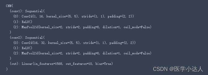
把模型实例化打印一下：

cnn=CNN()
print(cnn)

结果：

 开始训练：

# 添加优化方法
optimizer=torch.optim.Adam(cnn.parameters(),lr=LR)
# 指定损失函数使用交叉信息熵
loss_fn=nn.CrossEntropyLoss()
 
 
'''
开始训练我们的模型哦
'''
step=0
for epoch in range(EPOCH):
    #加载训练数据
    for step,data in enumerate(train_loader):
        x,y=data
        #分别得到训练数据的x和y的取值
        b_x=Variable(x)
        b_y=Variable(y)
 
        output=cnn(b_x)         #调用模型预测
        loss=loss_fn(output,b_y)#计算损失值
        optimizer.zero_grad()   #每一次循环之前，将梯度清零
        loss.backward()         #反向传播
        optimizer.step()        #梯度下降
 
        #每执行50次，输出一下当前epoch、loss、accuracy
        if (step%50==0):
            #计算一下模型预测正确率
            test_output=cnn(test_x)
            y_pred=torch.max(test_output,1)[1].data.squeeze()
            accuracy=sum(y_pred==test_y).item()/test_y.size(0)
 
            print('now epoch :  ', epoch, '   |  loss : %.4f ' % loss.item(), '     |   accuracy :   ' , accuracy)
 
'''
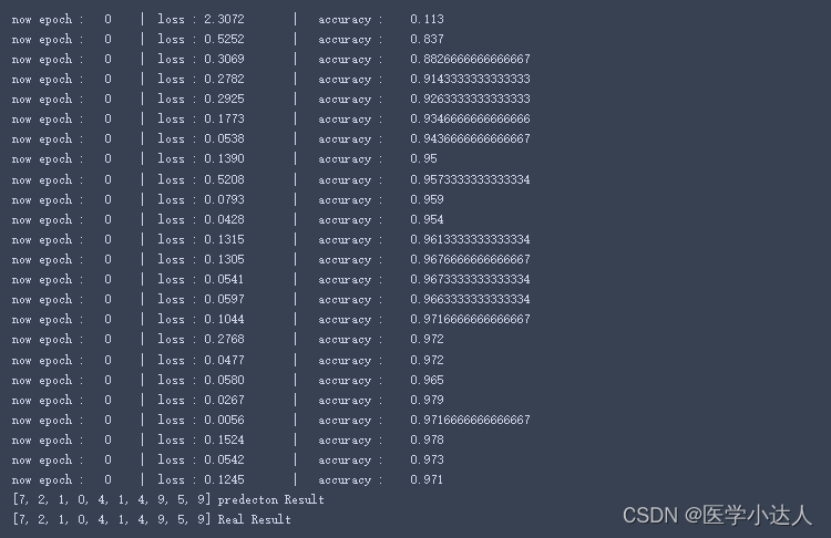
打印十个测试集的结果
'''
test_output=cnn(test_x[:10])
y_pred=torch.max(test_output,1)[1].data.squeeze()       #选取最大可能的数值所在的位置
print(y_pred.tolist(),'predecton Result')
print(test_y[:10].tolist(),'Real Result')

结果：

 卷积层维度变化：

（1）输入1*28*28，即1通道，28*28维；

（2）卷积层-01：16*28*28，即16个卷积核，卷积核维度5*5，步长1，边缘填充2，维度计算公式B = (A + 2*P - K) / S + 1，即（28+2*2-5）/1 +1 = 28

（3）池化层：池化层为2*2，所以输出为16*14*14

（4）卷积层-02：32*14*14，即32卷积核，其它同卷积层-01

(5) Pooling layer: The pooling layer is 2*2, so the output is 32*7*7;

(6) fc layer: Since the output is 1*10, that is, the probability of 10 categories, first compress the final pooling layer into two-dimensional (1, 32*7*7), and then the fully connected layer dimension (32 *7*7, 10), finally (1, 32*7*7)*(32*7*7, 10)