Sliding mode control quick start

posted on 2023-06-06 17:43 read(979) comment(0) like(1) collect(2)

0. Introduction

Recently, the author was invited and asked me to help explain sliding mode control to the juniors who are just getting started . But the author doesn't know how to explain these basic knowledge to the students who are not getting started, so the author flipped through the good articles and videos written in recent years. Taken together, let's summarize a set of relatively basic articles that are suitable for beginners. Here we first post the notes of Wang Chongwei .
insert image description here
The corresponding video link is below:

【Advanced Control Theory】17

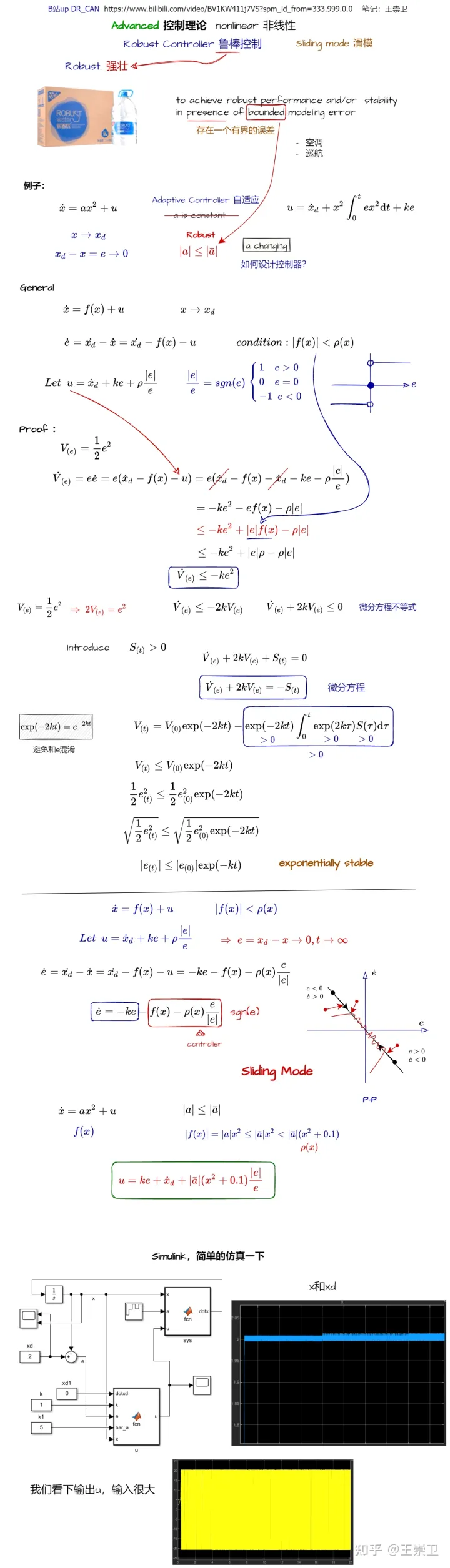
1. Purpose of sliding mode control

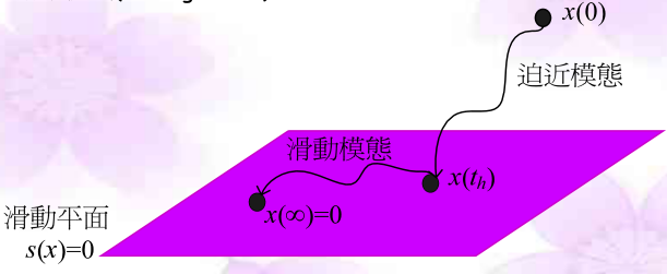
For sliding mode control, I think we need to understand its purpose before learning. At the beginning, our definition of sliding control is: sliding mode is a technology that first uses the controlled system to generate more than two subsystems, and then deliberately adds some switching conditions to generate sliding mode to achieve the control goal.

Sliding mode control (sliding mode control, SMC ) is also called variable structure control, which is a special kind of nonlinear control in essence, and nonlinearity is manifested as discontinuity of control. The difference between this control strategy and other controls is that the "structure" of the system is not fixed, but can be continuously changed in a dynamic process according to the current state of the system (such as deviation and its derivatives, etc.), Force the system to move according to the state trajectory of the predetermined "sliding mode".

For example sliding surfaces exist in sliding mode control $s = 0$ , in the beginning, the system will reach the sliding surface in a finite time, and then it will move along the sliding surface. In the theoretical formulation of the sliding mode, the system is constrained to the sliding surface, so it is only necessary to consider the system as sliding on the sliding surface. However, the realization of the actual system is to use high-frequency switching to make the system approximately slide on the sliding surface. The control signal of high-frequency switching allows the system to chatter within a range very close to the sliding surface, and its frequency is not fixed. Although the overall system is nonlinear, in the figure below, when the system reaches the sliding surface, the ideal (no jump) system will be limited to $s = 0$ On the sliding surface of , the sliding surface is a linear time-invariant system that is exponentially stable at the origin.
insert image description here

2. Advantages and disadvantages of sliding mode control

2.1 Advantages of sliding mode control:

The sliding mode can be designed and has nothing to do with object parameters and disturbances. It has fast response, insensitivity to parameter changes and disturbances (robustness), no need for online system identification, and simple physical implementation .

2.2 Disadvantages of sliding mode control:

When the state trajectory reaches the sliding mode surface, it is difficult to slide strictly along the sliding mode towards the equilibrium point, but it approaches the equilibrium point by crossing back and forth on both sides , resulting in chattering—the main problem in the practical application of sliding mode control. obstacle. At home and abroad , the purpose of reducing chattering is mainly achieved by improving the reaching law of the sliding mode .

3. Sliding mode control requires conditions

As mentioned above, the design of the sliding mode variable structure controller also includes two parts. One is that it can reach the sliding mode surface in a limited time from any position in the state space. $s = 0$ , and the second is that it can converge to the origin (balance point) on the sliding surface. This also means that we need to have a stable sliding surface, and the sliding surface is reachable. There are four conditions for this:

Stability condition: On the sliding mode surface of s=0, the state is convergent, that is, the sliding mode exists;
Accessibility condition: moving points outside the switching surface s=0 will reach the switching surface within a limited time;
Ensure the stability of sliding mode motion;
Meet the motion quality requirements of the control system.

The following will describe how to design a sliding mode control controller according to the four conditions. Part of the content here is based on the article Sliding Mode Control (Sliding Mode Control) and written with the author's understanding.

3.1 Sliding surface generation of the controlled system

The first step is that we need to understand that we need to find a sliding surface to keep the controlled system stable on the sliding surface.
For example, suppose there is a controlled system:

\begin{aligned} {\dot{x}}_{1} & = x_{2} \\ {\dot{x}}_{2} & = in \end{aligned}

$\begin{aligned} \dot{x}_1 &= x_2 \\ \dot{x}_2 &= u \end{aligned}$

\overset{x}{˙}_{1} \overset{x}{˙}_{2} = x_{2} = in

At this time, we need to design a sliding mode surface according to the controlled system. The sliding mode surface can generally be designed as the following form
$\sum_{i=1}^{n-1} c_i x_i + x_n$
Because in sliding mode control, it is necessary to ensure that the polynomial $p^{n − 1} + c_n p^{n − 2} + \cdots + c_2 p + c_1$ For Hurwitz (simply speaking, this condition is to satisfy the state in $s = 0$ can converge on the sliding surface).

What is Hurwitz, that is, the real part of the eigenvalue of the above polynomial is in the left half plane, which is negative.

We can see that there are two variables in the above-mentioned controlled system, so we need to take $n = 2$ ,Right now $s ( x ) = c_1 x_1 + x_2$ , in order to ensure that the polynomial $p+c_1$ For Hurwitz, the polynomial is required $p+c_1=0$ The real part of the eigenvalue of is negative, that is, $c_1>0$ .

We know that sliding mode control needs to make the state $x_1$ and $x_2$ The derivatives of all reach zero, we make $s = 0$ , analyze the result
$\left\{$
$\begin{aligned} c x_{1} + x_{2} = 0 \\ {\dot{x}}_{1} = x_{2} \end{aligned}$ $\begin{aligned} &cx_1 + x_2 = 0 \\ &\dot{x}_1 = x_2 \end{aligned}$ \right. ~~ \Rightarrow ~~ c x_1 + \dot{x}_1 = 0 ~~ \Rightarrow ~~ \left\{ $\begin{aligned} x_{1} (t) = {It is}^{- c t} x_{1} (0) \\ x_{2} (t) = {\dot{x}}_{1} (t) = - c x_{1} (0) {It is}^{- c t} \end{aligned}$ $\begin{aligned} &x_1(t) = \text{e}^{-ct} x_1(0) \\ &x_2(t) = \dot{x}_1(t) = -c x_1(0) \text{e}^{-ct} \end{aligned}$ \right. ${c x_{1} + x_{2} = 0 \overset{x}{˙}_{1} = x_{2} \Rightarrow c x_{1} + \overset{x}{˙}_{1} = 0 \Rightarrow {x_{1} (t) = It is^{- c t} x_{1} (0) x_{2} (t) = \overset{x}{˙}_{1} (t) = - c x_{1} (0) and^{- c t}$
The status can be seen through the above formula $x_1$ and $x_2$ Both eventually tend to zero, and the speed is tightening at an exponential rate. Exponential rate means that when $t = 1/ c$ , the process of going to zero is completed $63.2\%$ ,when $t = 3/ c$ , the process of going to zero is completed $95.021\%$ . Then we adjust the parameters $c$ The size can realize the adjustment of the zero speed, $c$ The bigger it is, the faster it is.

Therefore if satisfied $s=cx_1 + x_2=0$ , then the state of the system $x_1$ and $x_2$ will also approach zero along the sliding surface ( $s = 0$ called the sliding surface).

3.2 Design of reachability controller

After getting the sliding surface, it proves that the stability condition of the controlled system is established, and the next step is the accessibility condition, that is, the state $x$ Starting from any point in the state space, it can be reached in finite time $s = 0$ On the sliding surface of , we can use the Lyapunov indirect method to analyze at this time, as we can see from the front, the switching function $s$ is the state variable $x$ function, take the following Lyapunov function

$\frac{1}{2} s^2$

Time derivative can be obtained

\begin{aligned} \dot{IN} & = s \dot{s} \\ = s (- sgn (s) - s) \\ = - sgn (s) s - s^{2} \\ = - (| s | + s^{2}) < 0 \end{aligned}

$\begin{aligned} \dot{V} &= s \dot{s} \\ &= s (-\text{sgn}(s) - s) \\ &= -\text{sgn}(s) s - s^2 \\ &= -(|s| + s^2) < 0 \end{aligned}$

\dot{IN} = s \overset{s}{˙} = s (- sgn (s) - s) = - sgn (s) s - s^{2} = - (∣ s ∣ + s^{2}) < 0

To make the system stable, we need to make $\dot{V}<0$ ,Right now $\dot{s}<0$ . At this time the system for $s$ is asymptotically stable, there is no guarantee that its finite time to $s = 0$ on the sliding surface (asymptotically stable is when $t$ As it tends to infinity, the state variable $x$ tend to $0$ , that is, arrives in infinite time), so we need $\dot{s}<-\sigma$ , $\sigma$ is a very small positive number. $condition\color{red}{The above is the necessary basis for the establishment of the accessibility condition}$ .

But in fact, every design cannot always be judged by the Lyapunov function , so people put forward the concept of reaching law. The commonly used reaching laws are as follows, among which $\text{sgn}(s)$ is a symbolic function, $s>0,\text{sgn}(s)=1; s<0, \text{sgn}(s)=-1; s=0, \text{sgn}(s)=0$ :

Constant speed approach law: $\dot{s} = -\epsilon ~\text{sgn}(s), ~~~~\epsilon >$
Exponential reaching law: $\dot{s} = -\epsilon ~\text{sgn}(s) - k s, ~~~~\epsilon > 0, k>0$
Power reaching law: $\dot{s} = -k |s|^\alpha ~\text{sgn}(s) - k s, ~~~~k>0, 0<\alpha<1$

Generally, we need to complete the adjustment of these parameters during use. Generally, we use the exponential approach rate, and set $\epsilon$ and $k$ The values of are all set to 1, which simplifies to:

$\dot{s} = ~\text{sgn}(s) - s$

Then we know $s ( x ) = c_1 x_1 + x_2$ ,but $\dot{s} = ~\text{sgn}(s) - s = c_1 \dot{x_1} + \dot{x_2} = c_1x_2+u$ . Then we can get the controller $in$ for: