foreword

AI painting woke up from the DeepDream nightmare of 18 years, and in 2022 OpenAI 's DALL·E 2 achieved amazing results, as shown in the picture:

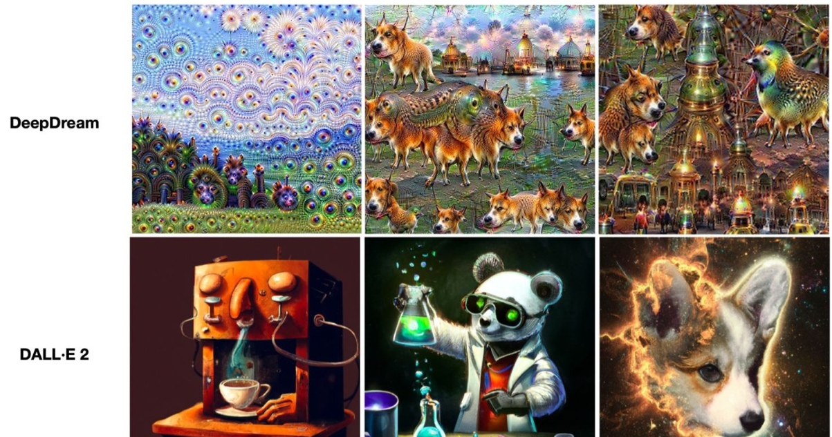
AI + art involves Transformer , VAE, ELBO, Diffusion Model and a series of knowledge related to mathematics. Diffusion Models are as complex as VAE .

Diffusion model (paper: DDPM stands for Denoising Diffusion Probabilistic Model) has received less attention since it was published in 2020, because it is not as simple and crude as GAN, but it has become so popular recently that more than half of the relevant submissions to ICRL conferences, and its two most advanced Text generation image - OpenAI's DALL·E 2 and Google's Imagen are both based on the diffusion model.

1. Common generative models

First horizontally compare several important generative models GAN, VAE , Flow-based Models, Diffusion Models.

GAN consists of a generator (generator) and a discriminator (discriminator), the generator is responsible for generating realistic data to "cheat" the discriminator, and the discriminator is responsible for judging whether a sample is real or "fabricated". The training of GAN is actually two models learning from each other. Can it not be called "confrontation" and be more harmonious.

VAE also hopes to train a generative model x=g(z) , which can map the sampled probability distribution to the probability distribution of the training set , generate a hidden variable z , and z contains both data information and noise, except for restoring the input In addition to the sample data, it can also be used to generate new data.

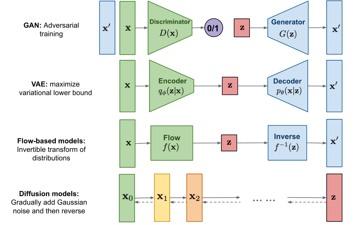
Diffusion Models are inspired by non-equilibrium thermodynamics (non-equilibrium thermodynamics) . The theory first defines a Markov chain of diffusion steps to slowly add random noise to the data, and then learns the reverse diffusion process to construct the desired data samples from the noise . Unlike VAE or flow models, diffusion models are learned through a fixed process, and the latent space z has relatively high dimensionality.

2. Intuitive understanding of Diffusion model

A generative model is essentially a set of probability distributions. As shown in the figure, the left side is a training data set, and all the data in it are random samples taken independently and identically distributed from a certain data p _{data .} On the right is its generative model (probability distribution). In this probability distribution, find a distribution p _θ that makes it the closest to the p _data . Then take new samples on p _{θ to obtain a steady stream of new data.}

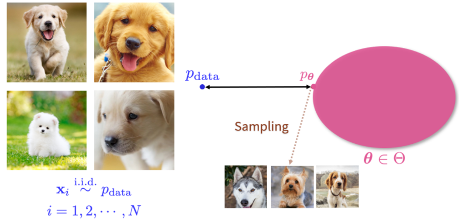
However, the form of p _data is often very complex, and the dimension of the image is very high, it is difficult for us to traverse the entire space, and the data samples we can observe are also limited.

Diffusion function :

We can add noise to any distribution, including the p _data we are interested in, so that it eventually becomes a pure noise distribution N(0,I) . How do you understand it?

From the perspective of probability distribution , consider the two-dimensional joint probability distribution p(x,y) of the Swiss roll shape in the figure below . The diffusion process q is very intuitive. The originally concentrated and orderly sample points are disturbed by noise and diffuse outward. Eventually becomes a completely disordered noise distribution.

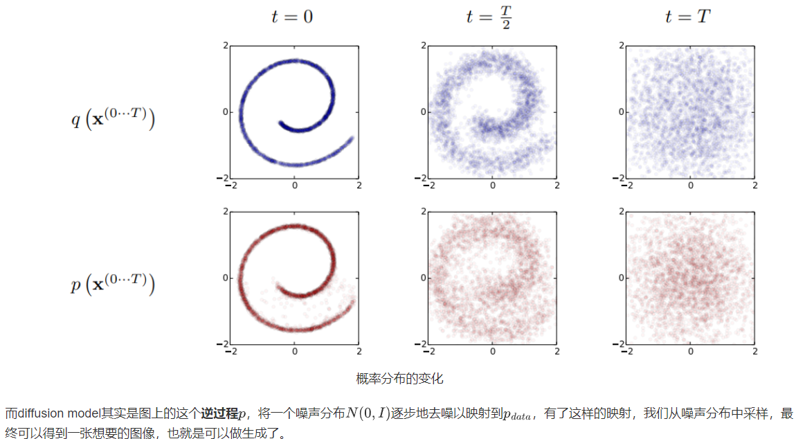
Looking at this process from a single image sample , the diffusion process q is to continuously add noise to the image until the image becomes a pure noise, and the inverse diffusion process p is the process of generating an image from pure noise. Sample changes:

3. Formal analysis of Diffusion model

Since it is called a generative model, it means that Diffusion Models are used to generate data similar to the training data . Fundamentally, Diffusion Models work by corrupting the training data by continuously adding Gaussian noise, and then learning to restore the data by reversing this noise process.

When testing, you can use Diffusion Models to feed randomly sampled noise into the model and learn the denoising process to generate data . That is the basic principle corresponding to the figure below.

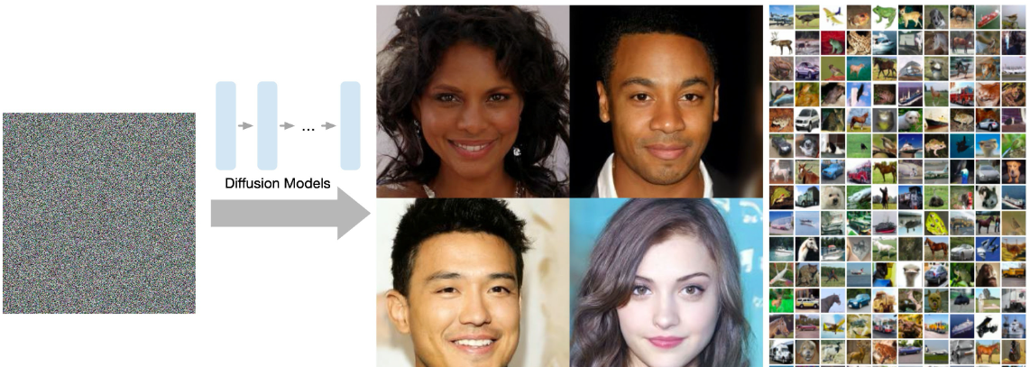
More specifically, the diffusion model is a latent variable model that maps to latent space using a Markov Chain (MC). Through the Markov chain, noise is gradually added to the data xi at each time step t _to obtain the posterior probability q(x _1:T | x ₀ ) , where x ₁ …x _T represents the input data and is also latent space. That is to say, the latent space of Diffusion Models has the same dimension as the input data.

Posterior probability : In Bayesian statistics, the posterior probability of a random event or an uncertain event is the conditional probability obtained after considering and giving relevant evidence or data. wiki

A Markov chain is a random process in state space that goes through transitions from one state to another. This process requires the property of "no memory": the probability distribution of the next state can only be determined by the current state, and the events before it in the time series have nothing to do with it .

Diffusion Models are divided into forward diffusion process and reverse reverse diffusion process. The figure below shows the diffusion process. From the end to the end is a Markov chain, which represents the random process of transition from one state to another in the state space. The subscript is the image diffusion process corresponding to Diffusion Models.

Finally, the real image input from x ₀ is asymptotically transformed into a pure Gaussian noise image x _T after Diffusion Models .

Model training mainly focuses on the inverse diffusion process. The goal of training a diffusion model is to learn the inverse of the forward process: the training probability distribution p _θ (x _t-1 | x _t ) . By traversing backwards along the Markov chain, new data x ₀ can be regenerated .

The biggest difference between Diffusion Models and GAN or VAE is that it is not generated by a model, but based on the Markov chain, which generates data by learning noise.

In addition to generating high-quality images, another advantage of Diffusion Models is that there is no confrontation during the training process . For the GAN network model, confrontational training is actually very difficult to debug, because the two models that compete with each other during the confrontation training process, It's a black box for us. In addition, in terms of training efficiency, the diffusion model is also scalable and parallelizable , so how to speed up the training process, how to add more mathematical rules and constraints, and expand to voice, text, and 3D fields is very interesting. Lots of new articles.

*4. Detailed explanation of Diffusion Model (mathematical derivation)

It has been clearly stated above that Diffusion Models consist of a forward process (or diffusion process) and a reverse process (or reverse diffusion process), in which the input data is gradually noised, and then the noise is converted back to a sample of the source target distribution. The principle is Markov chain + conditional probability distribution . The core is how to use the neural network model to solve the probability distribution of the Markov process.

1. Forward process (diffusion process)

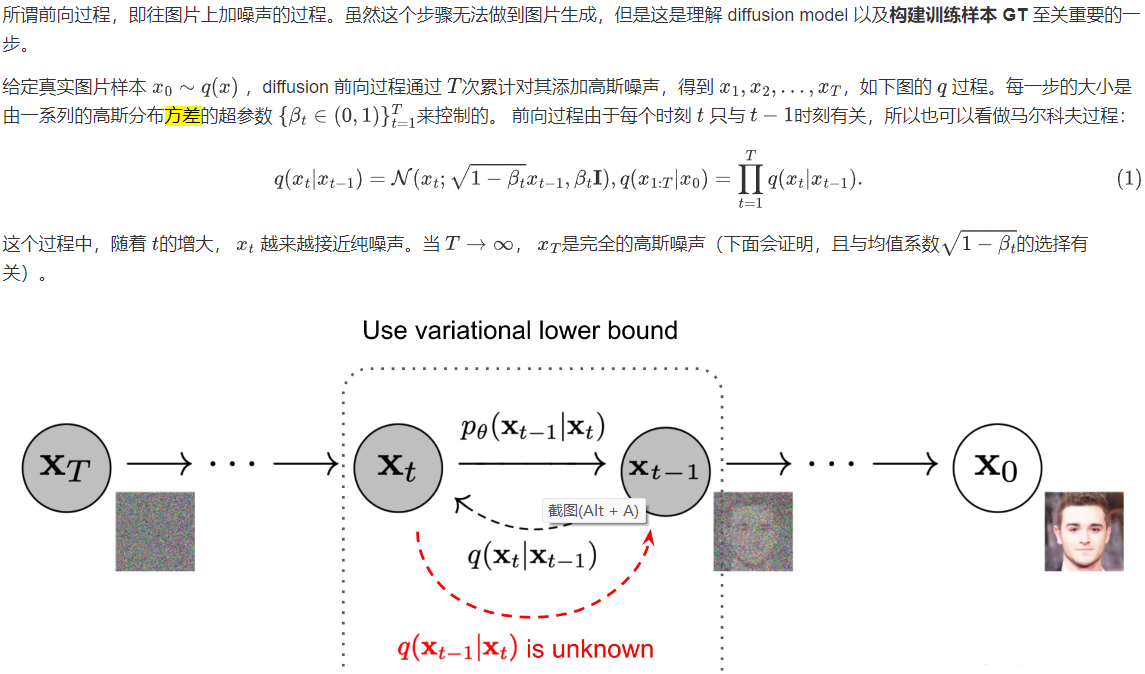
Two important properties to use during implementation and derivation:

Feature 1: Reparameterization trick
The reparameter technique has been cited in many works (gumbel softmax, VAE). If we want to randomly sample a sample (Gaussian distribution) from a certain distribution, this process cannot reverse the gradient. And this process of obtaining x _t through Gaussian noise sampling is everywhere in diffusion, so we need to use heavy parameter techniques to make it differentiable:

_{Property 2: x t} at any time can be represented by x ₀ and β _t

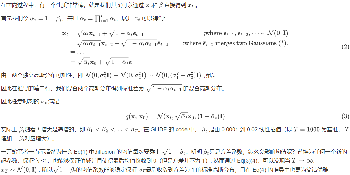
2. Inverse Diffusion Process

If the forward process (forward) is the process of adding noise, then the reverse process (reverse) is the denoising process of diffusion.

If we can reverse the above process and sample from q(x _t-1 |x _t ) , we can restore the original image distribution x ₀ ~q(x ) from Gaussian noise x _{T ~N( 0, I ).} It is proved in Document 7 that if q(x _t |x _t-1 ) satisfies a Gaussian distribution and β _t is small enough, q(x _t-1 |x _t ) is still a Gaussian distribution. However, we cannot simply infer q(x _t-1 |x _t ) , so we use a deep learning model (the parameter is θ, the current mainstream is U-Net+attention structure) to predict such a reverse distribution p θ ( _similar to VAE):

However, in the paper, the author directly takes the variance of the conditional probability p _θ (x _t-1 |x _t ) as β _t , instead of the Σ _θ (x _t , t) that needs to be estimated by the network as mentioned above, so the actual Only the mean needs to be estimated by the network.

The forward diffusion and reverse diffusion processes are both Markov, then normal distribution, and then step by step conditional probability. The only difference is that the mean and variance of the Gaussian distribution of each conditional probability in forward diffusion have been determined ( Depends on β _t and x ₀ ), and the mean and variance in the inverse diffusion process are what our network needs to learn.

3. Inverse diffusion conditional probability derivation

Although we can't get the probability distribution q(x _t-1 |x _t ) of the reversal process , if we know x ₀ , q(x _t-1 |x _t , x ₀ ) can be written directly. This thing is probably such a form

Bayesian formula:

into the formula to get:

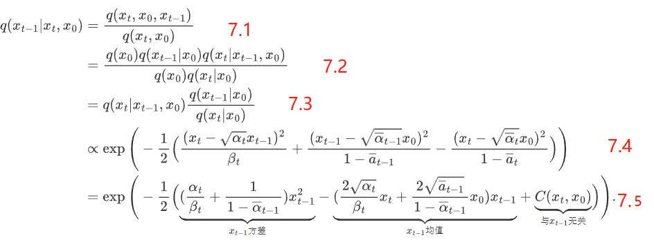
7-1 is brought into the Bayesian formula 2; 7-2 is brought into the multiplication formula 1, and then we can get 7-3

The probability density function of univariate normal distribution is defined as:
, which can be substituted into Equation 7.4

Equation 7.5 can be organized as$\frac{1}{2}$(ax ² +bx+c), that is$\frac{1}{2}$a (x+ $\frac{b}{2a\_}$) ² +C, whose mean is -$\frac{b}{2a\_}$, with a variance of$\frac{1}{a}$, so we can get the variance and mean in (6) after a little tidying up:

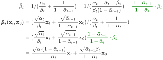
According to the formula (2) of characteristic 2, we know that , into the above formula:

It can be seen that under the condition of given x _{0 ,} the mean value of the posterior conditional Gaussian distribution is only related to the hyperparameters, x _t and ε _t , and the variance is only related to the hyperparameters.

Through the above variance and mean, we get the analytical form of q(x _t-1 |x _t , x ₀ ) .

4. Training Loss

_{How to train Diffusion Models to obtain the mean value μ θ} (x _t , t) and variance Σ _θ (x _t , t) in formula (3) ? In VAE, we have learned the role of maximum likelihood estimation: for the real training sample data known, the parameters of the model are required, and maximum likelihood estimation can be used.

In statistics, the likelihood function is a function of the parameters of a statistical model. Given the output x, the likelihood function L(θ|x) with respect to the parameter θ is (numerically) equal to the probability of the variable X given the parameter θ: L(θ|x)=P(X=x|θ) .

Diffusion Models uses maximum likelihood estimation to find the probability distribution of Markov chain conversion in the process of inverse diffusion, which is the training purpose of Diffusion Models. That is, to maximize the log likelihood of the model prediction distribution, from the perspective of Loss decline is to minimize the negative log likelihood:

The process is much like a VAE, i.e. the negative log-likelihood can be optimized using a variational lower bound (VLB) .

KL divergence is an asymmetric statistical distance measure used to measure the degree of difference between one probability distribution P and another probability distribution Q. The mathematical form of the KL divergence of a continuous distribution is:

Properties of the KL divergence:

From the KL divergence we know:

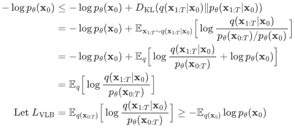
Further, the upper bound of the cross-entropy of the above formula can be written, and the upper bound can be further simplified:

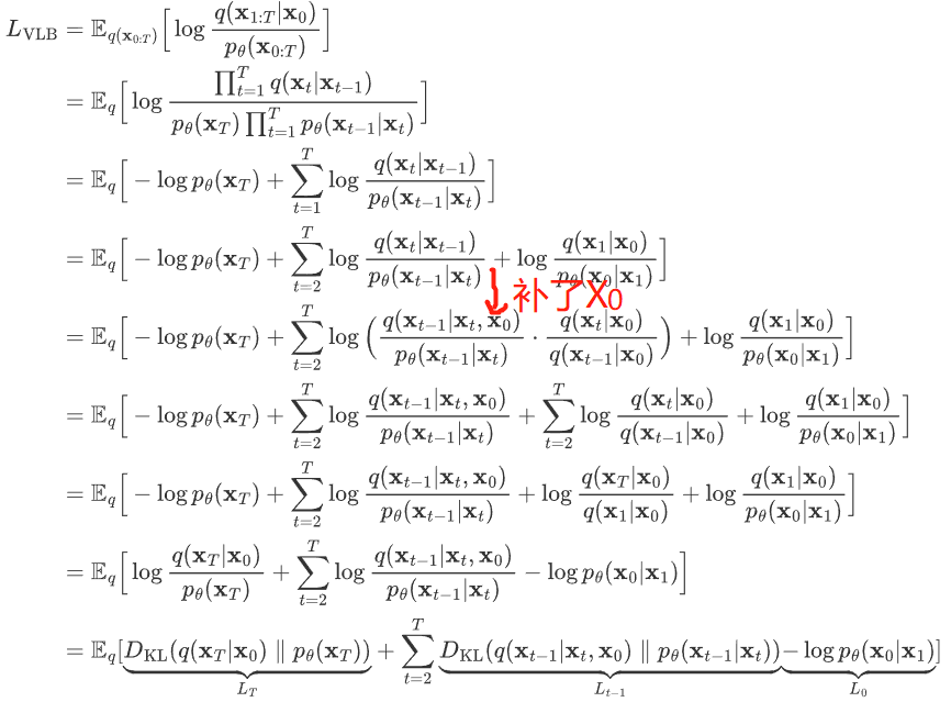
Next, we classify and discuss these three situations:

First, since the forward process q has no learnable parameters, and x _T is pure Gaussian noise, L _T can be ignored as a constant.

Then, L _t-1 is the KL divergence, which can be regarded as shortening the distance between the two distributions:

1. 第一个分布 q(x_t-1|x_T,x₀,) 我们已经在上一节推导出其解析形式，这是一个高斯分布，其均值和方差为
   
2. 第二个分布 p_θ(x_t-1，x_t) 是我们网络期望拟合的目标分布，也是一个高斯分布，均值用网络估计，方差被设置为了一个和 β_t 有关的常数。
   
   如果有两个分布 p,q 都是高斯分布，则他们的KL散度为
   
   然后因为这两个分布的方差全是常数，和优化无关，所以其实优化目标就是两个分布均值的二范数
   
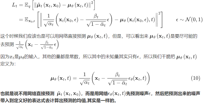
   把这个公式，带入到 上一公式中得到：
   
   经过这样一番推导之后就是个 L2 loss。网络的输入是一张和噪声线性组合的图片，然后要估计出来这个噪声：
   

五、训练、测试伪代码

1. 训练

2.测试

六、代码解析

推荐一个简易ddpm项目，用cifar10数据集进行训练：
github.com/abarankab/DDPM
使用代码请见：

1.train_cifar.py

from torchvision import datasets

# 1.定义模型（Unet，后续会展开）
diffusion = script_utils.get_diffusion_from_args(args).to(device)
diffusion.load_state_dict(torch.load(args.model_checkpoint))  

# 2.迭代器
optimizer = torch.optim.Adam(diffusion.parameters(), lr=args.learning_rate)

# 3.从 torchvision 读入数据集
train_dataset = datasets.CIFAR10( root='./cifar_train', train=True,
            download=True, transform=script_utils.get_transform())
train_loader = script_utils.cycle(DataLoader( train_dataset,  batch_size=batch_size, shuffle=True, drop_last=True,num_workers=-1,))


for iteration in range(1, 80000):
        diffusion.train()
        x, y = next(train_loader)

        if args.use_labels:
            loss = diffusion(x, y)
        else:
            loss = diffusion(x)

展开1：定义 diffusion

model = UNet(img_channels=3, base_channels=128)
    
# 生成 t=1000 对应的 β（0.001~0.02）
if args.schedule == "cosine":
    betas = generate_cosine_schedule(args.num_timesteps=1000)
else:
    betas = generate_linear_schedule(num_timesteps=1000,
        1e-4 * 1000 / args.num_timesteps,
        0.02 * 1000 / args.num_timesteps)

diffusion = GaussianDiffusion( model, (32, 32), 3, 10, betas,
    ema_decay=0.9999,  ema_update_rate=1, ema_start=2000, loss_type='l2')
    
return diffusion

展开2：UNet
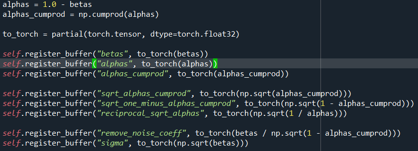
由 time_mlp、init_conv(3,128)、down（12层ResidualBlock）、mid、up（12层Res）组成。time_mlp为 时间步 t 的可学习张量，下面有具体定义代码；
GaussianDiffusion为预设的一系列超参数，如 β、累乘α等：

class PositionalEmbedding(nn.Module):
    __doc__ = r"""Computes a positional embedding of timesteps.

    Input:
        x: tensor of shape (N)
    Output:
        tensor of shape (N, dim)
    Args:
        dim (int): embedding dimension
        scale (float): linear scale to be applied to timesteps. Default: 1.0
    """

    def __init__(self, dim, scale=1.0):
        super().__init__()
        assert dim % 2 == 0
        self.dim = dim
        self.scale = scale

    def forward(self, x):
        device = x.device
        half_dim = self.dim // 2
        emb = math.log(10000) / half_dim
        emb = torch.exp(torch.arange(half_dim, device=device) * -emb)
        emb = torch.outer(x * self.scale, emb)
        emb = torch.cat((emb.sin(), emb.cos()), dim=-1)
        return emb

self.time_mlp = nn.Sequential(
            PositionalEmbedding(base_channels=128, time_emb_scale=1.0),
            nn.Linear(128, 512),
            nn.SiLU(),
            nn.Linear(512, 512),
        )

展开3：loss = diffusion(x)

b, c, h, w = x.shape                    # x:128，3，32，32  y是对应的128个标签

t = torch.randint(0, self.num_timesteps, (b,), device=device) 
# 从(0,1000)中随机选128个t

return self.get_losses(x, t, y)
def get_losses(self, x, t, y):
    noise = torch.randn_like(x)         # 随机噪声

    1.perturbed_x = self.perturb_x(x, t, noise)    
      # 用x0表示出xt， 下一行是具体操作：
      perturbed_x = extract(self.sqrt_alphas_cumprod, t, x.shape) * x + 
                    extract(self.sqrt_one_minus_alphas_cumprod, t, x.shape) * noise

    2.estimated_noise = self.model(perturbed_x, t, y)
      # 下一行是具体操作：
      2.1. time_emb = self.time_mlp(t)         # (128) -> (128,512)
           emb = math.log(10000) / half_dim    # 10000/64= 0.143
           emb = torch.exp(torch.arange(half_dim, device=device) * -emb)    # (64):[1.0, 0.86, 0.75, ...0.0001]
           emb = torch.outer(t * self.scale, emb)        # (128,64) 矩阵乘法
           emb = torch.cat((emb.sin(), emb.cos()), dim=-1)   # （128，128）
           time_emb = conv2d(emb)              # (128,512)
      
      2.2. for layer in self.downs:
               x = layer(x, time_emb, y)    # 将 time_emb 添加到特征中。即：
               out += self.time_bias(self.activation(time_emb))[:, :, None, None]
               # self.time_bias 是linear（512，128），activation 是silu函数。直接跟特征相加
           for layer in self.mid:
               x = layer(x, time_emb, y)
           for layer in self.ups:
               x = layer(x, time_emb, y)

           x = self.activation(self.out_norm(x))
           x = self.out_conv(x)              # 返回值为噪音（跟输入维度相同）

           
    
    if self.loss_type == "l1":
        loss = (estimated_noise - noise).abs().mean()
    elif self.loss_type == "l2":
        loss = (estimated_noise - noise).square().mean()

    return loss

2.sample_images.py（预测过程）

x = torch.randn(batch_size, self.img_channels, *self.img_size, device=device)
# 随机采样高斯噪声，作为xt

for t in range(self.num_timesteps - 1, -1, -1):        # T=1000
    t_batch = torch.tensor([t], device=device).repeat(batch_size)  
    x = self.remove_noise(x, t_batch, y, use_ema)      # 得到x(t-1),即：
    x = (    (x - extract(self.remove_noise_coeff, t, x.shape) * self.model(x, t, y)) 
         * extract(self.reciprocal_sqrt_alphas, t, x.shape)       )

最后一行代码，即

总结

1. Diffusion Model 通过参数化的方式表示为马尔科夫链，这意味着隐变量 x₁,…x_T 都满足当前时间步 t 只依赖于上一个时间步 t-1，这样对后续计算很有帮助。
2. 马尔科夫链中的转变概率分布 p_θ(x_t-1|x_t) 服从高斯分布，在正向扩散过程当中高斯分布的参数是直接设定的，而逆向过程中的高斯分布参数是通过学习得到的。
3. Diffusion Model 网络模型扩展性和鲁棒性比较强，可以选择输入和输出维度相同的网络模型，例如类似于UNet的架构，保持网络模型的输入和输出 Tensor dims 相等。
4. Diffusion Model 的目的是对输入数据求极大似然函数，实际表现为通过训练来调整模型参数以最小化数据的负对数似然的变分上限
5. In the process of probability distribution conversion, because of the Markov assumption, the variational upper limit in the fourth point of the objective function can be converted to use KL divergence to calculate, so the method of Monte Carlo sampling is avoided.