In this issue, the cases are more hard-core. It is suitable for masters of science and engineering, and students of humanities and social sciences can read the previous cases.

case background

This article was published last year, and the publication was also printed. Now I share some code as a case for students who need it.

Original text link (HowNet article C core):

A Lithium Battery Life Prediction Method Based on Mode Decomposition and Machine Learning

Li-ion battery remaining useful life (RUL) is an important indicator of battery health management. This paper uses battery capacity as an indicator of health status, and uses modal decomposition and machine learning algorithms to propose a CEEMDAN-RF-SED-LSTM method to predict the RUL of lithium batteries.

First, CEEMDAN is used to decompose the battery capacity data. In order to avoid the influence of the noise in the fluctuation component on the prediction ability of the model, and not completely discard the characteristic information in the fluctuation component, this work proposes to use the random forest (RF) algorithm to obtain the value of each fluctuation component. Importance ranking and numerical value, which are used as the weight of each component for the explanatory power of the original data. Then, the prediction results obtained by the weight value and the neural network model constructed by different fluctuation components are weighted and reconstructed, and then the RUL prediction of the lithium-ion battery is obtained.

The article compares the prediction accuracy of a single model and a combined model. The prediction accuracy of the combined model with RF has further improved the performance of the five neural networks. The performance test of this method is carried out with the NASA dataset as the research object. The experimental results show that the CEEMDAN-RF-SED-LSTM model has a good performance in predicting battery RUL, and the prediction results have lower errors than a single model.

The above is a summary. I won’t introduce the principles. They are all in the article. This blog is mainly to share a process of how to use these neural networks to build time series forecasting. Just some code , not the whole code of this article.

It mainly uses modal decomposition to decompose the battery capacity degradation curve, then uses random forest regression to adjust the weight coefficient of the modal component, and finally uses the neural network to predict and add. The codec structure behind the article is this blog. No.

Data Sources

NASA's battery data set is very old. NASA seems to have removed this data set last year. However, there are still many acquisition methods on the Internet. Of course, the original data is stored in matlab files, and it needs to be processed and cleaned before it can be extracted and used.

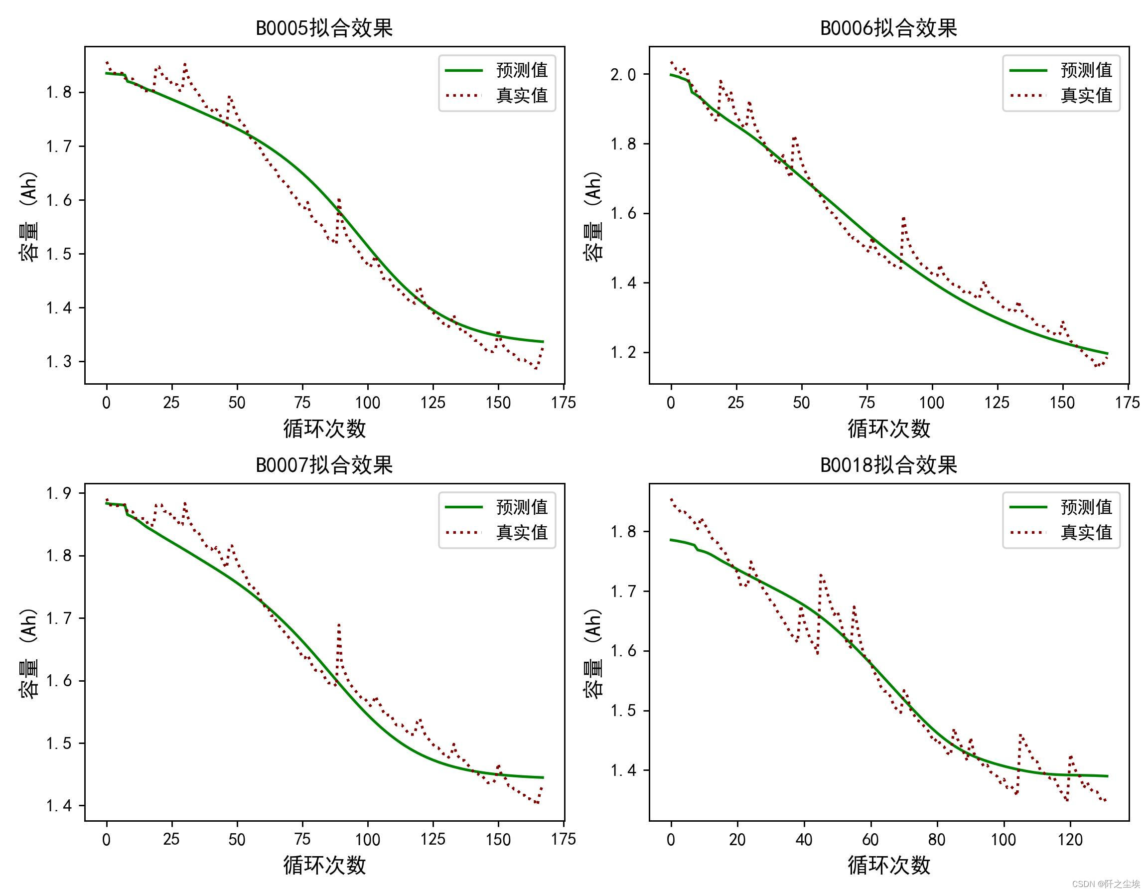
In the article, all 4 batteries have been tested. This blog uses the data of one battery, B0006, as a demonstration.

Deep Learning Framework 

The Keras framework based on TensorFlow is used, which is easy to get started. Although pytorch is very popular in academia, object-oriented programming really makes it difficult for programming novice to understand. .

Code implementation preparation

Since it is the code of a relatively systematic article, my code style here will have a clear division of labor, has an engineering nature, and has a high degree of encapsulation. In order to facilitate reuse, there will be a large number of package adjustments and custom functions, which must be programmed Only the basics of thinking can be understood, and it is not as simple as the previous cases.

Import required packages

import os
import math
import datetime
import random as rn
import numpy as np
import pandas as pd
import matplotlib.pyplot as plt
%matplotlib inline
plt.rcParams ['font.sans-serif'] ='SimHei'               #显示中文
plt.rcParams ['axes.unicode_minus']=False               #显示负号
 
from PyEMD import EMD,CEEMDAN,Visualisation 
 
from sklearn.model_selection import train_test_split
from sklearn.preprocessing import MinMaxScaler
from sklearn.ensemble import RandomForestRegressor
from sklearn.metrics import mean_absolute_error
from sklearn.metrics import mean_squared_error
 
import tensorflow as tf
import keras
from keras.models import Model, Sequential
from keras.layers import GRU, Dense,Conv1D, MaxPooling1D,GlobalMaxPooling1D,Embedding,Dropout,Flatten,SimpleRNN,LSTM
#from keras.callbacks import EarlyStopping
#from tensorflow.keras import regularizers
#from keras.utils.np_utils import to_categorical
from tensorflow.keras  import optimizers

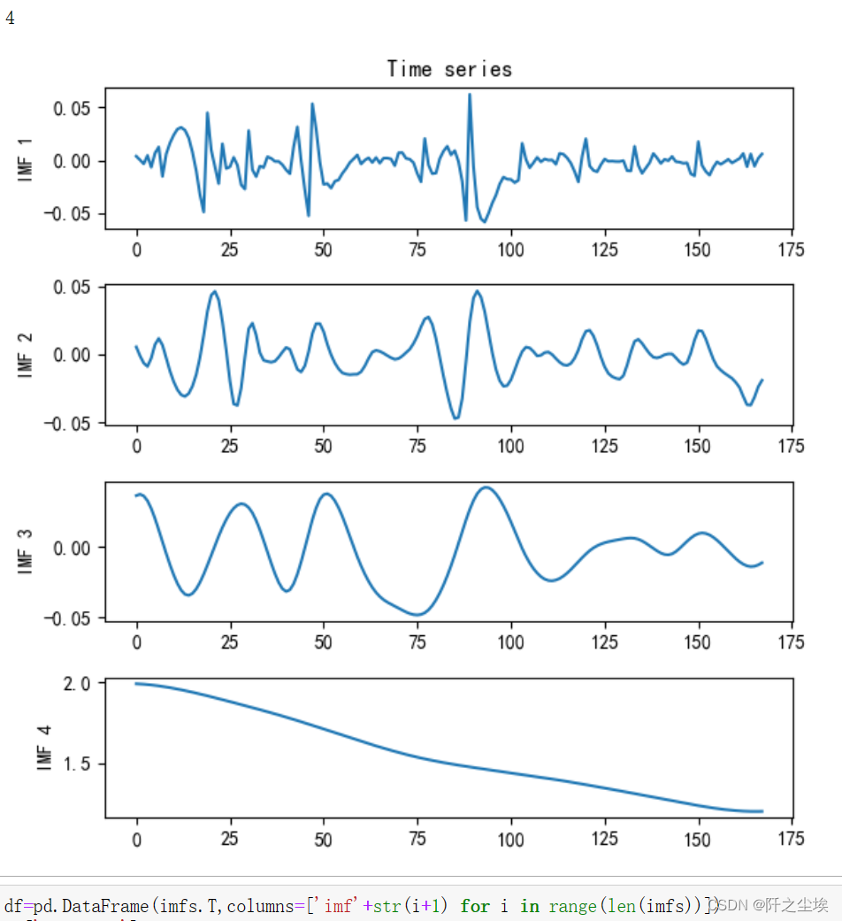
Read the data, perform CEEMDAN modal decomposition, and then draw a picture to view the decomposition results:

data0=pd.read_csv('NASA电容量.csv',usecols=['B0006'])
S1 = data0.values
S = S1[:,0]
t = np.arange(0,len(S),1)  
ceemdan=CEEMDAN()
ceemdan.ceemdan(S)
imfs, res = ceemdan.get_imfs_and_residue()
print(len(imfs))
vis = Visualisation()
vis.plot_imfs(imfs=imfs, residue=res, t=t , include_residue=False)

The 4 below is the number of modes representing the decomposition. 

 Perform random forest regression on 4 modes:

df=pd.DataFrame(imfs.T,columns=['imf'+str(i+1) for i in range(len(imfs))])
df['capacity']=data0.values
X_train=df.iloc[:,:-1]
y_train=df.iloc[:,-1]
model = RandomForestRegressor(n_estimators=5000, max_features=2, random_state=0)
model.fit(X_train, y_train)
model.score(X_train, y_train)

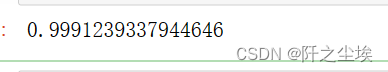
Goodness of fit 99.9% 

plot variable importance

model.feature_importances_
sorted_index = model.feature_importances_.argsort()
plt.barh(range(X_train.shape[1]), model.feature_importances_[sorted_index])
plt.yticks(np.arange(X_train.shape[1]), X_train.columns[sorted_index])
plt.xlabel('Feature Importance')
plt.ylabel('Feature')
plt.title('Random Forest')
plt.tight_layout()

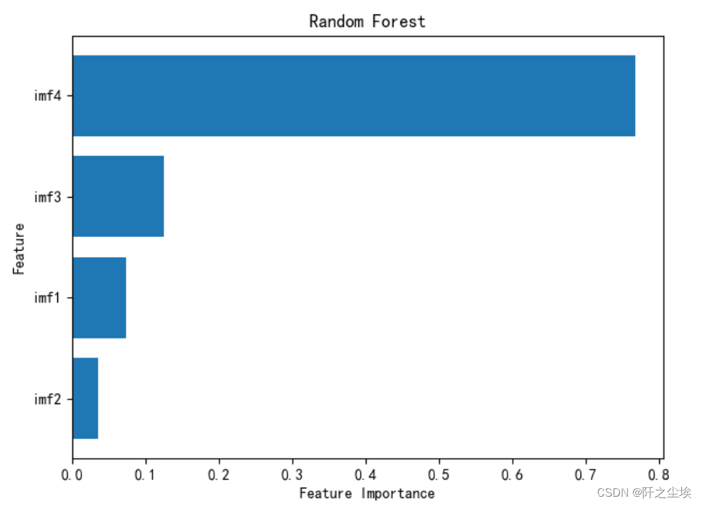
 Note component names and importance:

imf_names=X_train.columns[sorted_index][::-1]
imf_weight=model.feature_importances_[sorted_index][::-1]
imf_weight[0]=1
#imf_names,imf_weight

Define random number seed function, error evaluation index calculation function

def set_my_seed():
    os.environ['PYTHONHASHSEED'] = '0'
    np.random.seed(1)
    rn.seed(12345)
    tf.random.set_seed(123)
    
def evaluation(y_test, y_predict):
    mae = mean_absolute_error(y_test, y_predict)
    mse = mean_squared_error(y_test, y_predict)
    rmse = math.sqrt(mean_squared_error(y_test, y_predict))
    mape=(abs(y_predict -y_test)/ y_test).mean()
    return mae, rmse, mape
 
def relative_error(y_test, y_predict, threshold):
    true_re, pred_re = len(y_test), 0
    for i in range(len(y_test)-1):
        if y_test[i] <= threshold >= y_test[i+1]:
            true_re = i - 1
            break
    for i in range(len(y_predict)-1):
        if y_predict[i] <= threshold:
            pred_re = i - 1
            break
    return abs(true_re - pred_re)/true_re

Define the function to construct the sequence, and obtain the explanatory variables and response variables corresponding to the training set and test set from the sequence data

def build_sequences(text, window_size=4):
    #text:list of capacity
    x, y = [],[]
    for i in range(len(text) - window_size):
        sequence = text[i:i+window_size]
        target = text[i+window_size]
        x.append(sequence)
        y.append(target)
    return np.array(x), np.array(y)
def get_traintest(data,train_size=len(data0),window_size=4):
    train=data[:train_size]
    test=data[train_size-window_size:]
    X_train,y_train=build_sequences(train,window_size=window_size)
    X_test,y_test=build_sequences(test)
    return X_train,y_train,X_test,y_test

Define the function to build the model, as well as the function to draw the loss graph, and the fitting effect evaluation and comparison function:

def build_model(X_train,mode='LSTM',hidden_dim=[32,16]):
    set_my_seed()
    model = Sequential()
    if mode=='RNN':
        #RNN
        model.add(SimpleRNN(hidden_dim[0],return_sequences=True, input_shape=(X_train.shape[-2],X_train.shape[-1])))
        model.add(SimpleRNN(hidden_dim[1]))     
        
    elif mode=='MLP':
        model.add(Dense(hidden_dim[0],activation='relu',input_shape=(X_train.shape[-1],)))
        model.add(Dense(hidden_dim[1],activation='relu'))
        
    elif mode=='LSTM':
        # LSTM
        model.add(LSTM(hidden_dim[0],return_sequences=True, input_shape=(X_train.shape[-2],X_train.shape[-1])))
        model.add(LSTM(hidden_dim[1]))
    elif mode=='GRU':
        #GRU
        model.add(GRU(hidden_dim[0],return_sequences=True, input_shape=(X_train.shape[-2],X_train.shape[-1])))
        model.add(GRU(hidden_dim[1]))
    elif mode=='CNN':
        #一维卷积
        model.add(Conv1D(hidden_dim[0],3,activation='relu',input_shape=(X_train.shape[-2],X_train.shape[-1])))
        model.add(GlobalMaxPooling1D())
        
    model.add(Dense(1))
    model.compile(optimizer='Adam', loss='mse',metrics=[tf.keras.metrics.RootMeanSquaredError(),"mape","mae"])
    return model
 
def plot_loss(hist,imfname):
    plt.subplots(1,4,figsize=(16,2))
    for i,key in enumerate(hist.history.keys()):
        n=int(str('14')+str(i+1))
        plt.subplot(n)
        plt.plot(hist.history[key], 'k', label=f'Training {key}')
        plt.title(f'{imfname} Training {key}')
        plt.xlabel('Epochs')
        plt.ylabel(key)
        plt.legend()
    plt.tight_layout()
    plt.show()
    
def evaluation_all(df_RFW_eval_all,df_eval_all,mode,Rated_Capacity=2,show_fit=True):
    df_RFW_eval_all['all_pred']=df_RFW_eval_all.iloc[:,1:].sum(axis=1)
    df_eval_all['all_pred']=df_eval_all.iloc[:,1:].sum(axis=1)
 
    MAE1,RMSE1,MAPE1=evaluation(df_RFW_eval_all['capacity'],df_RFW_eval_all['all_pred'])
    RE1=relative_error(df_RFW_eval_all['capacity'],df_RFW_eval_all['all_pred'],threshold=Rated_Capacity*0.7)
 
    MAE2,RMSE2,MAPE2=evaluation(df_eval_all['capacity'],df_eval_all['all_pred'])
    RE2=relative_error(df_eval_all['capacity'],df_eval_all['all_pred'],threshold=Rated_Capacity*0.7)
 
    df_RFW_eval_all.rename(columns={'all_pred':'predict','capacity':'actual'},inplace=True)
    if show_fit:
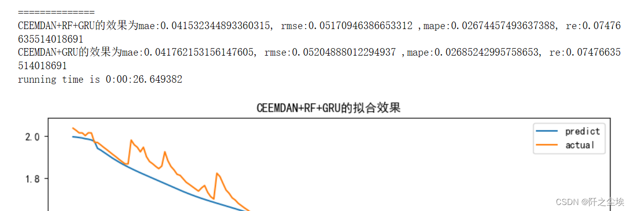
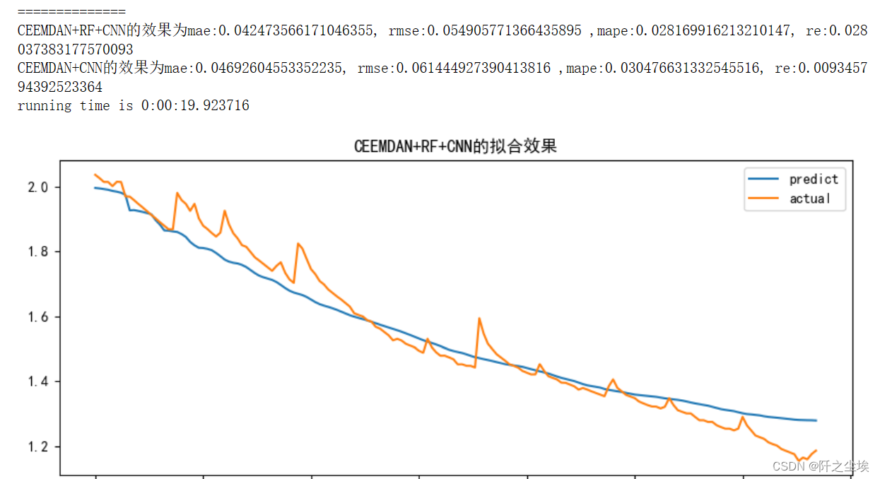
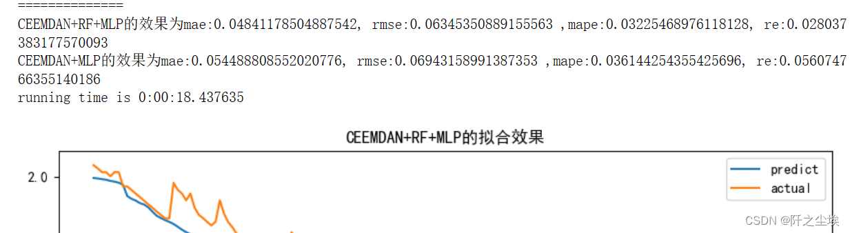
        df_RFW_eval_all.loc[:,['predict','actual']].plot(figsize=(10,4),title=f'CEEMDAN+RF+{mode}的拟合效果')
 
    print(f'CEEMDAN+RF+{mode}的效果为mae:{MAE1}, rmse:{RMSE1} ,mape:{MAPE1}, re:{RE1}')
    print(f'CEEMDAN+{mode}的效果为mae:{MAE2}, rmse:{RMSE2} ,mape:{MAPE2}, re:{RE2}')

Define the training function

def train_fuc(mode='LSTM',window_size=8,batch_size=32,epochs=100,hidden_dim=[32,16],Rated_Capacity=2,show_imf=False,show_loss=True,show_fit=True):
    df_RFW_eval_all=pd.DataFrame(df['capacity'])
    df_eval_all=pd.DataFrame(df['capacity'])
    for i,imfname in  enumerate(imf_names):
 
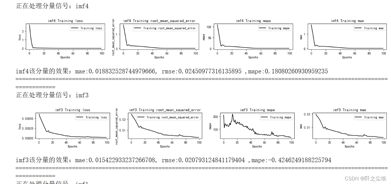
        print(f'正在处理分量信号：{imfname}')
        data=df[imfname]
        X_train,y_train,X_test,y_test=get_traintest(data.values,window_size=window_size,train_size=len(data))
        if mode!='MLP':
            X_train = X_train.reshape((X_train.shape[0], X_train.shape[1], 1))
        #print(X_train.shape, y_train.shape)
        start = datetime.datetime.now()
        set_my_seed()
        model=build_model(X_train=X_train,mode=mode,hidden_dim=hidden_dim)
        hist=model.fit(X_train, y_train,batch_size=batch_size,epochs=epochs,verbose=0)
        if show_loss:
            plot_loss(hist,imfname)
        #预测
        point_list = list(data[:window_size].values.copy())
        y_pred=[]
        while (len(point_list)) < len(data.values):
            x = np.reshape(np.array(point_list[-window_size:]), (-1, window_size)).astype(np.float32)
            pred = model.predict(x) 
            next_point = pred[0,0]
            point_list.append(next_point)#加入原来序列用来继续预测下一个点
            #point_list.append(next_point)#保存输出序列最后一个点的预测值
        y_pred.append(point_list)#保存本次预测所有的预测值
        y_pred=np.array(y_pred).T
        #print(y_pred.shape)
        end = datetime.datetime.now()
        
        if show_imf:
            df_eval=pd.DataFrame()
            df_eval['actual']=data.values
            df_eval['pred']=y_pred
        mae, rmse, mape=evaluation(y_test=data.values, y_predict=y_pred)
        print(f'{imfname}该分量的效果：mae:{mae}, rmse:{rmse} ,mape:{mape}')
        df_eval_all[imfname+'_w_pred']=y_pred
        df_RFW_eval_all[imfname+'_w_pred']=y_pred*imf_weight[i]
        print('============================================================================================================================')
    evaluation_all(df_RFW_eval_all,df_eval_all,mode=mode,Rated_Capacity=Rated_Capacity,show_fit=show_fit)
    print(f'running time is {end-start}')

The training function uses all the previous custom functions, and I want to understand the functions of all the custom functions. 

The values ​​of the initialization parameters are the default values ​​of the hyperparameters.

window_size=8
batch_size=16
epochs=100
hidden_dim=[32,16]
Rated_Capacity=2
show_fit=True
show_loss=True
mode='LSTM'  #RNN,GRU,CNN

 window_size refers to the size of the sliding sequence window

batch_size is the batch size

epochs is the number of training epochs

hidden_dim is the number of neurons in the hidden layer of the neural network

Rated_Capacity is the initial value of the battery capacity, the initial value of the battery in NASA is 2

show_fit Whether to display the fitting effect graph

show_loss Whether to display the loss change graph

mode is the neural network model type

Model Training and Evaluation

The above code encapsulates all the processes, and the next training and evaluation only need to change the parameters.

LSTM prediction

mode='LSTM' 
set_my_seed()
train_fuc(mode=mode,window_size=window_size,batch_size=batch_size,epochs=epochs,hidden_dim=hidden_dim,Rated_Capacity=Rated_Capacity)

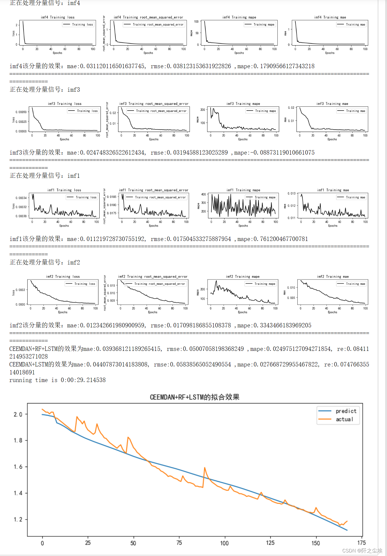
The output effect is as above, it will print the change of training loss of each component, the evaluation index of point estimation, and the final evaluation index of the overall prediction effect with random forest and without random forest.

(My anaconda has been reinstalled once before, the environment has changed, and the value in the paper can't be run out...but the difference is not big, for example, mae, here is 0.039368, the paper is 0.039161, and other indicators are similar)

If you want to change other parameters, just change them directly in the sequence function. For example, if you want to use a sliding window of 16:

train_fuc(window_size=16)

You can run it to get the result. If the picture is too long, it will not be cut.

The default model in my training function is LSTM (because it works best)

If you want to change the number of neurons in the hidden layer, you can write it like this:

train_fuc(hidden_dim=[64,32])

Very concise and convenient.

 RNN prediction

Just modify the mode parameter

mode='RNN' 
set_my_seed()
train_fuc(mode=mode,window_size=window_size,batch_size=32,epochs=epochs,hidden_dim=hidden_dim,Rated_Capacity=Rated_Capacity)

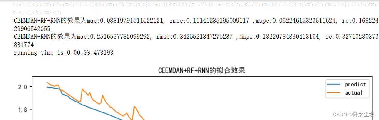
 The picture is too long so I won’t finish it, just look at the results of the final evaluation index calculation. (The same is true, because the running environment has been reinstalled, so the current running results are slightly different from those in my thesis)

(Screenshot of the paper)

 GRU forecast

mode='GRU' 
set_my_seed()
train_fuc(mode=mode,window_size=window_size,batch_size=batch_size,epochs=epochs,hidden_dim=hidden_dim,Rated_Capacity=Rated_Capacity)

1D CNN prediction

mode='CNN' 
set_my_seed()
train_fuc(mode=mode,window_size=window_size,batch_size=batch_size,epochs=epochs,hidden_dim=hidden_dim,Rated_Capacity=Rated_Capacity)

MLP forecast

mode='MLP' 
set_my_seed()
train_fuc(mode=mode,window_size=window_size,batch_size=batch_size,epochs=90,hidden_dim=hidden_dim,Rated_Capacity=Rated_Capacity)

I didn't spend too much time adjusting other hyperparameters, because the neural network takes a long time to run at a time. If students are interested, they can try more hyperparameter adjustments, and maybe they can get better prediction results.

Pictures in my article: