News from this site

Rental advertising space, please contact the webmaster if you need cooperation

article

27841

browse

+focus

classification

no classification

date

2024-11(5)

多目标进化算法——NSGA-II（python实现）

posted on 2023-06-03 19:27 read(768) comment(0) like(24) collect(0)

foreword

Since NSGA-II is based on genetic algorithm, before explaining NSGA-II , we first have some basic understanding of genetic algorithm - genetic algorithm is often used in single-objective optimization problems, the basic process of operation is as follows

Cross-mutation by the binary value of the solution yields different solutions
According to the fitness function, the fitness value of each solution is obtained
Sort and filter the current solution set according to the size of the fitness value.
Then carry out a new round of cross-mutation on the selected individuals, and repeat the cycle to make the solution set more and more close to the real optimization goal.

What NSGA-II does is actually change the basis of sorting——It is "how to judge the quality of a solution". In the traditional genetic algorithm, the value of the fitness function is used . This is also because the traditional genetic algorithm is mostly used in single-objective optimization problems. Using this indicator can be used to judge .
The following is the corresponding relationship of some nouns in the genetic algorithm:

mathematical concepts	biological concept
current set of solutions	current population
Each solution in the solution set	individuals in a population

NSGA-II

But for a multi-objective optimization problem, its optimal solution is no longer a value, but a Pareto front in a multidimensional space: a collection of optimal solutions. Therefore, for the solutions that do not reach the Pareto front in the iterative process, judging their pros and cons should start from two aspects -
Convergence - The degree (or speed)
distribution of the solution close to the Pareto front - Whether the current solution set is as close as possible to the Pareto front Possibly covered to the pareto front.
Therefore, Deb, the author of NSGA-II, proposed two indicators to evaluate the pros and cons of the current solution set:

non-dominated sort
Sort by crowding distance

In the following, for the convenience of explanation, we take the minimization optimization problem of dual objectives as an example, because this can help us understand it in a two-dimensional plane in a geometric sense.
$\quad F(x)=\{f_1(x),f_2(x)\}^T\\ st. \quad x\in X \\ \quad \quad X \subset\mathbb R^2$

non-dominated sort

dominance relationship

First, it is necessary to understand the dominance relationship between the two solutions. Let's take an example to illustrate that if both objectives are minimization objectives, the smaller the value of the objective function, the better. Then assume
that a given individual $x_0$ ,
the objective function value $F(x_0) =(f_1(x_0),f_2(x_0))=(1,1)$
given another individual $x_1$ ,
the objective function value $F(x_1) =(f_1(x_1),f_2(x_1))=(2,2)$
We can find that, in the two objective function directions (objective), $x_0$ The desired value of the objective function $(1, 1)$ all than $x_1$ The objective function value of $(2, 2)$ is small, while both optimization directions are minimized. so $x_0$ The resulting solution is better than $x_1$ ,Right now $x_0$ dominate $x_1$ .
Similarly, when one direction is equal, the dominance relationship is determined by the value of the objective function in the other direction, for example: $(1, 2)$ dominate $(2, 2)$ .
If it is understood in a geometric sense on a two-dimensional plan view, it is to make concentric circles from the origin to the outside, and the points on the inner circle dominate the points on the outer circle. (Of course, it is limited to two objectives, and the optimization direction is to minimize)

non-dominant relationship

But we will encounter another situation, such as $(1, 2)$ and $(2, 1)$ , obviously in one direction 2 > 1, but in the other direction 1 < 2, corresponding to the geometric sense, that is, these two points are on the same circle. When there is no clear dominance relationship like this, that is, when the two parties cannot dominate each other, the relationship between the two is a non-domination relationship.
To sum up, for two individuals, their size relationship can correspond to their dominance relationship. So in the class definition, I overloaded the less than sign method to facilitate the comparison of the dominance relationship between two individuals in the code.

    # 重载小于号“<”
    def __lt__(self, other):
        v1 = list(self.objective.values())
        v2 = list(other.objective.values())
        for i in range(len(v1)):
            if v1[i] > v2[i]:
                return 0  # 但凡有一个位置是 v1大于v2的 直接返回0,如果相等的话比较下一个目标值
        return 1

non-dominated sorting algorithm

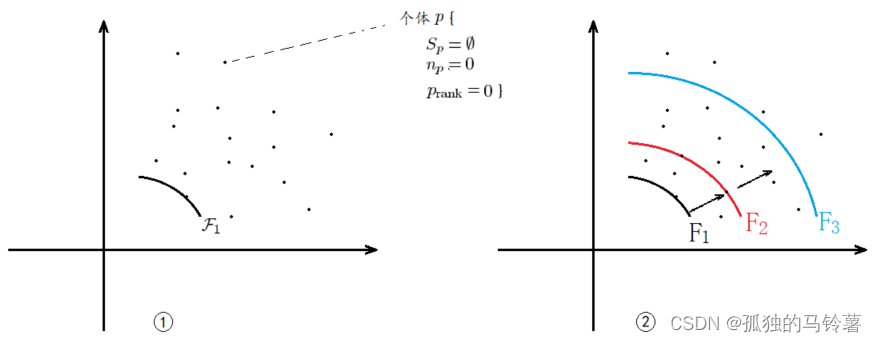
algorithm thinking

From the above, it is obvious that the dominance relationship can be used as an indicator to measure the quality of the solution, so we use the dominance relationship between individuals to stratify the existing population. The solution closest to the Pareto front has the highest rank and is the first layer. Then determine which layer each individual is in in turn, and assign a rank to each individual. From a geometric point of view, it is similar to drawing concentric circles, and see which concentric circle the solution is in. Then sort and select according to the rank value of each individual.

Algorithm Pseudocode

The following is the pseudocode of the original author:
insert image description here

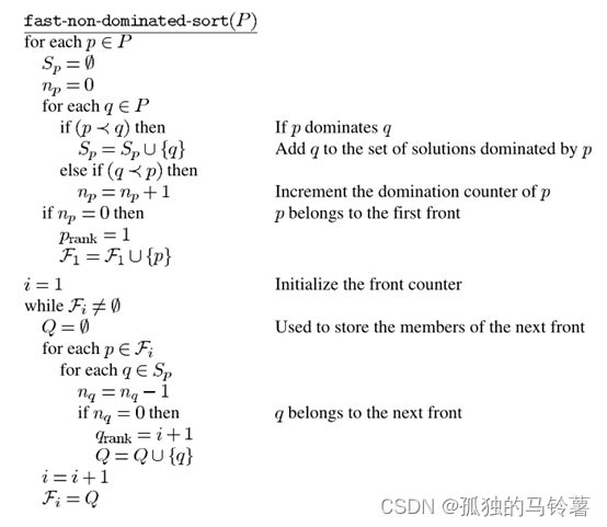
Pseudocode Interpretation

Here you need to understand the meaning of several of the variables——
$n_p$ :untie $p$ Dominated by several solutions, it is a value (the number of points in the lower left part)
$S_p$ :untie $p$ Which solutions dominate, is a set of solutions (the content of the upper right part of the point)
$F_i$ : No. $i$ The solution set of the layer (obviously, the solutions in the same layer are mutually non-dominated solutions)
$p_{rank}$ :untie $p$ The level of the layer (the smaller the better)
pseudocode is mainly carried out in two steps:

all individual $n_p$ , $S_p$ All have been calculated, but only the rank of the most advanced individual is determined, and the rank value of all individuals in this layer is set to 1, and then put into the $F_1$ layer.
use $F_1$ Middle individual $p$ of $S_p$ (the following points are placed inside), take each individual $q(\in S_p)$ , each time the individual is dominated by p in the previous layer, the individual attribute $n$ The value is reduced by 1. Then, when the layer's $p$ have dominated $q$ After one time, if $n_p =0$ . illustrate $q$ is the next layer immediately adjacent to this layer, then put $q$ put into a $F_2$ in the individual $q$ The attribute rank = 2
Repeat the steps of 2. for $F_2$ ,get $F_3$ ,...

Python code implementation

def fast_non_dominated_sort(P):
    """
    非支配排序
    :param P: 种群 P
    :return F: F=(F_1, F_2, ...) 将种群 P 分为了不同的层， 返回值类型是dict，键为层号，值为 List 类型，存放着该层的个体
    """
    F = defaultdict(list)

    for p in P:
        p.S = []
        p.n = 0
        for q in P:
            if p < q:  # if p dominate q
                p.S.append(q)  # Add q to the set of solutions dominated by p
            elif q < p:
                p.n += 1  # Increment the domination counter of p
        if p.n == 0:
            p.rank = 1
            F[1].append(p)

    i = 1
    while F[i]:
        Q = []
        for p in F[i]:
            for q in p.S:
                q.n = q.n - 1
                if q.n == 0:
                    q.rank = i + 1
                    Q.append(q)
        i = i + 1
        F[i] = Q

    return F

transition 1

The non-dominated sorting method described above measures the quality of the solution from the convergence of the solution, or the degree to which it is close to the frontier of Pareto. Based on this, we assume that there are 120 individuals in the population to be selected, and our population size is 100, that is, we need to select the first 100 as parents to enter the next iteration.
By non-dominated sorting, if get $F_1$ There are 30, $F_2$ There are 60, $F_3$ There are 10, $F_4$ There are 20 of them. Obviously, we only choose $F_1$ , $F_2$ , $F_3$ Individuals in will do. But the above situation is just right, we need to consider the more general situation -
if the dividing line is cut at $F_i$ layer, that is, if $F_3$ There are 30, and we need to choose 10 of them and exclude 20. How to choose in this case? That is, for individuals in the same layer with the same rank attribute value, what should we sort them by?

Sort by crowding distance

algorithm thinking

Therefore, in order to ensure the diversity of the population, that is, to preserve the sparseness of the distribution of the solution, the author tries to disperse the solution as much as possible when viewed on the graph. Under this principle, the solutions located at both ends must be kept, and the points in the middle are judged by defining the crowding distance. To understand it more vividly, it is "there are too many similar people around you who are relatively close, and it is enough to leave you as the only one who can represent this paragraph."

Algorithm Pseudocode

The following is the pseudo-code of the original author:
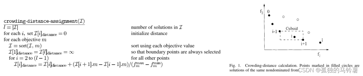insert image description here This code is relatively simple. In different target directions, the crowding distance of the two ends (the target value is the largest and the smallest) is directly set to positive infinity, and the middle point follows a formula. Briefly summarized as:

The crowding distance of a certain point = the sum of the normalized differences between the adjacent upper and lower points in different target directions

Python code implementation

def crowding_distance_assignment(L):
    """ 传进来的参数应该是L = F(i)，类型是List"""
    l = len(L)  # number of solution in F

    for i in range(l):
        L[i].distance = 0  # initialize distance

    for m in L[0].objective.keys():
        L.sort(key=lambda x: x.objective[m])  # sort using each objective value
        L[0].distance = float('inf')
        L[l - 1].distance = float('inf')  # so that boundary points are always selected

        # 排序是由小到大的，所以最大值和最小值分别是 L[l-1] 和 L[0]
        f_max = L[l - 1].objective[m]
        f_min = L[0].objective[m]

        for i in range(1, l - 1):  # for all other points
            L[i].distance = L[i].distance + (L[i + 1].objective[m] - L[i - 1].objective[m]) / (f_max - f_min)

        # 虽然发生概率较小，但为了防止除0错，当bug发生时请替换为以下代码
        # if f_max != f_min:
        #     for i in range(1, l - 1):  # for all other points
        #         L[i].distance = L[i].distance + (L[i + 1].objective[m] - L[i - 1].objective[m]) / (f_max - f_min)

transition 2

After introducing "non-dominated sorting" and "crowding distance allocation", the basic process of sorting selection for an existing population can be determined——

Given two individuals in the population, first compare their ranks, the smaller the value, the closer they are to the Pareto front, so choose the one with the smaller rank value.
If the rank values of the two individuals are the same, that is, when the two solutions are non-dominated solutions, compare their crowding_distance. The larger the value, the sparser the location and the more diverse the population, so choose a large crowding_distance value. of.

Binary Tournament

The above process is the basic strategy for the selection of " Dual Tournament ". (Binary Tournament: Randomly select two individuals, compare them according to a certain index strategy, and the better individual wins as one of the fathers for crossover)
The corresponding code is as follows

def binary_tournament(ind1, ind2):
    """
    二元锦标赛
    :param ind1:个体1号
    :param ind2: 个体2号
    :return:返回较优的个体
    """
    if ind1.rank != ind2.rank:  # 如果两个个体有支配关系，即在两个不同的rank中，选择rank小的
        return ind1 if ind1.rank < ind2.rank else ind2
    elif ind1.distance != ind2.distance:  # 如果两个个体rank相同，比较拥挤度距离，选择拥挤读距离大的
        return ind1 if ind1.distance > ind2.distance else ind2
    else:  # 如果rank和拥挤度都相同，返回任意一个都可以
        return ind1

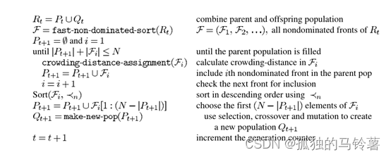
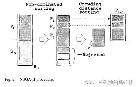
elite selection strategy

First of all, in the traditional genetic algorithm, in a certain iteration, only the parent generation of this iteration participates in the selection of cross mutation, so as to generate offspring as the parent generation of the next iteration.
In NSGA-II , in order to ensure that the optimal solution is not lost and improve the convergence speed of the algorithm, the author proposes an "elite selection strategy", that is, the parent $P_t$ and offspring $Q_t$ populations, merged into one population $R_t$ , perform non-dominated sorting and congestion distance calculation on the whole, sort and select as the next parent generation according to the above method $P_{t+1}$ . The parent generation is then selected and cross-sorted by the general method to generate offspring $Q_{t+1}$ .
This is also where the main process of the cycle is located!

insert image description here

Select crossover mutation to generate new population

choose

Randomly select two individuals from the population, let them go through the "dual tournament" mentioned in transition 2, and the winning one will be the male parent 1; do the same to get another male parent 2. Afterwards, in order to avoid the premature phenomenon in the genetic algorithm, an extra step of judgment is added to make the male parent 1 and the male parent 2 different.

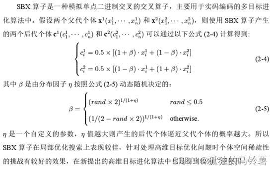
cross

The obtained two parents are crossed to produce two offspring. The crossover operator chosen here is "Simulated Binary Crossover (SBX)"
insert image description here

Mutations

For the two offspring obtained, one of them is mutated, and the other remains unchanged (do not change both, it will cause a premature phenomenon-all individuals are prematurely trapped in certain extreme values and stop changing , the specific reason is unknown, to be resolved), the mutation operator selected here is "polynomial mutation" (PM)
$x_j=x_j+ \Delta_j \\ ~\\ ~\\ \Delta_j =$

{\begin{cases} (2 m_{i})^{\frac{1}{the + 1}} & m_{i} < 0.5 \\ 1 - [2 (1 - m_{i})]^{\frac{1}{the + 1}} & m_{i} \geq 0.5 \end{cases}

$\begin{cases} (2\mu_i)^{\frac{1}{\eta + 1}} & \mu_i<0.5 \\ 1-[2(1-\mu_i)]^{\frac{1}{\eta + 1}} & \mu_i\ge0.5 \end{cases}$

xj​=xj​+Dj​  Dj​={( 2 mi​)h + 11​1−[ 2 ( 1−mi​) ]h + 11​​mi​<0.5 _ _mi​≥0.5 _ _​

\mu_i

is a random number that satisfies (0,1) uniform distribution,

\eta

is the variance distribution parameter.

Python code implementation

def make_new_pop(P, eta, bound_min, bound_max, objective_fun):
    """
    use select,crossover and mutation to create a new population Q
    :param P: 父代种群
    :param eta: 变异分布参数，该值越大则产生的后代个体逼近父代的概率越大。Deb建议设为 1
    :param bound_min: 定义域下限
    :param bound_max: 定义域上限
    :param objective_fun: 目标函数
    :return Q : 子代种群
    """
    popnum = len(P)
    Q = []
    # binary tournament selection
    for i in range(int(popnum / 2)):
        # 从种群中随机选择两个个体，进行二元锦标赛，选择出一个 parent1
        i = random.randint(0, popnum - 1)
        j = random.randint(0, popnum - 1)
        parent1 = binary_tournament(P[i], P[j])

        # 从种群中随机选择两个个体，进行二元锦标赛，选择出一个 parent2
        i = random.randint(0, popnum - 1)
        j = random.randint(0, popnum - 1)
        parent2 = binary_tournament(P[i], P[j])

        while (parent1.solution == parent2.solution).all():  # 如果选择到的两个父代完全一样，则重选另一个
            i = random.randint(0, popnum - 1)
            j = random.randint(0, popnum - 1)
            parent2 = binary_tournament(P[i], P[j])

        # parent1 和 parent1 进行交叉，变异 产生 2 个子代
        Two_offspring = crossover_mutation(parent1, parent2, eta, bound_min, bound_max, objective_fun)

        # 产生的子代进入子代种群
        Q.append(Two_offspring[0])
        Q.append(Two_offspring[1])
    return Q


def crossover_mutation(parent1, parent2, eta, bound_min, bound_max, objective_fun):
    """
    交叉方式使用二进制交叉算子（SBX），变异方式采用多项式变异（PM）
    :param parent1: 父代1
    :param parent2: 父代2
    :param eta: 变异分布参数，该值越大则产生的后代个体逼近父代的概率越大。Deb建议设为 1
    :param bound_min: 定义域下限
    :param bound_max: 定义域上限
    :param objective_fun: 目标函数
    :return: 2 个子代
    """
    poplength = len(parent1.solution)

    offspring1 = Individual()
    offspring2 = Individual()
    offspring1.solution = np.empty(poplength)
    offspring2.solution = np.empty(poplength)

    # 二进制交叉
    for i in range(poplength):
        rand = random.random()
        beta = (rand * 2) ** (1 / (eta + 1)) if rand < 0.5 else (1 / (2 * (1 - rand))) ** (1.0 / (eta + 1))
        offspring1.solution[i] = 0.5 * ((1 + beta) * parent1.solution[i] + (1 - beta) * parent2.solution[i])
        offspring2.solution[i] = 0.5 * ((1 - beta) * parent1.solution[i] + (1 + beta) * parent2.solution[i])

    # 多项式变异
    # TODO 变异的时候只变异一个，不要两个都变，不然要么出现早熟现象，要么收敛速度巨慢 why？
    for i in range(poplength):
        mu = random.random()
        delta = (2 * mu) ** (1 / (eta + 1)) if mu < 0.5 else (1 - (2 * (1 - mu)) ** (1 / (eta + 1)))
        offspring1.solution[i] = offspring1.solution[i] + delta

    # 定义域越界处理
    offspring1.bound_process(bound_min, bound_max)
    offspring2.bound_process(bound_min, bound_max)

    # 计算目标函数值
    offspring1.calculate_objective(objective_fun)
    offspring2.calculate_objective(objective_fun)

    return [offspring1, offspring2]

Overall flow chart

The above is all the required parts, and the following is to write the main function. When writing a program, you still have to look at the specific flow chart:
insert image description here
Therefore, the Python code of the main function part is implemented as follows:

def main():
    # 初始化/参数设置
    generations = 250  # 迭代次数
    popnum = 100  # 种群大小
    eta = 1  # 变异分布参数，该值越大则产生的后代个体逼近父代的概率越大。Deb建议设为 1

    poplength = 30  # 单个个体解向量的维数
    bound_min = 0  # 定义域
    bound_max = 1
    objective_fun = ZDT2

    # poplength = 3  # 单个个体解向量的维数
    # bound_min = -5  # 定义域
    # bound_max = 5
    # objective_fun = KUR

    # 生成第一代种群
    P = []
    for i in range(popnum):
        P.append(Individual())
        P[i].solution = np.random.rand(poplength) * (bound_max - bound_min) + bound_min  # 随机生成个体可行解
        P[i].bound_process(bound_min, bound_max)  # 定义域越界处理
        P[i].calculate_objective(objective_fun)  # 计算目标函数值

    # 否 -> 非支配排序
    fast_non_dominated_sort(P)
    Q = make_new_pop(P, eta, bound_min, bound_max, objective_fun)

    P_t = P  # 当前这一届的父代种群
    Q_t = Q  # 当前这一届的子代种群

    for gen_cur in range(generations):
        R_t = P_t + Q_t  # combine parent and offspring population
        F = fast_non_dominated_sort(R_t)

        P_n = []  # 即为P_t+1,表示下一届的父代
        i = 1
        while len(P_n) + len(F[i]) < popnum:  # until the parent population is filled
            crowding_distance_assignment(F[i])  # calculate crowding-distance in F_i
            P_n = P_n + F[i]  # include ith non dominated front in the parent pop
            i = i + 1  # check the next front for inclusion
        F[i].sort(key=lambda x: x.distance)  # sort in descending order using <n，因为本身就在同一层，所以相当于直接比拥挤距离
        P_n = P_n + F[i][:popnum - len(P_n)]
        Q_n = make_new_pop(P_n, eta, bound_min, bound_max,
                           objective_fun)  # use selection,crossover and mutation to create a new population Q_n

        # 求得下一届的父代和子代成为当前届的父代和子代，，进入下一次迭代 《=》 t = t + 1
        P_t = P_n
        Q_t = Q_n

        # 绘图
        plt.clf()
        plt.title('current generation:' + str(gen_cur + 1))
        plot_P(P_t)
        plt.pause(0.1)

    plt.show()

    return 0

Test function and result

Here, the test function uses ZDT1 (the paper also gives many other test functions, see TABLE1 in the original paper for details): the
insert image description here
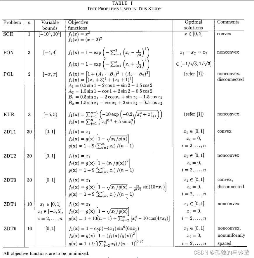
obtained results are as follows: