
YOLOv5训练结果分析
posted on 2023-05-07 21:22 read(425) comment(0) like(19) collect(1)
The purpose of this article is to help understand the series of files that appear under the runs/train folder after each training, and to explore how to evaluate the accuracy and the quality of the model.

1. Confusion matrix —confusion_matrix.png
The train run by Bi She has a confusion matrix, but it is a bit ridiculous. You need to run the bird to verify it (to be verified)
1. Concept
A confusion matrix is a summary of the predictions for a classification problem. Aggregating the number of correct and incorrect predictions using count values, broken down by each class, shows where the classification model confuses when making predictions.
The confusion matrix not only allows us to intuitively understand the mistakes made by the classification model, but more importantly, it can understand which types of errors are occurring. It is this decomposition of the results that overcomes the limitations of using only classification accuracy.
2. Graphical understanding
| actual | ||||
| class 1 | Class 2 | Class 3 | ||
| predict | class 1 | 43 | 5 | 2 |
| Class 2 | 2 | 45 | 3 | |
| Class 3 | 0 | 1 | 49 | |
(1) The horizontal axis is the predicted category, and the vertical axis is the real category;
(2) The total number in the table is 150, indicating that there are 150 test samples in total;
(3) The sum of each row is 50, which means that each class has 50 samples, and each row represents the number of real targets predicted as other classes. For example, the first row: 43 represents 43 of the real class 1. Predicted as class 1, 5 were mispredicted as class 2, and 2 were mispredicted as class 3;
2.TP/TN/FP/FN
1. Logical relationship
T(True): The final prediction is correct.
F (False): The final prediction result is wrong.
P (Positive): The model predicts that it is a positive example (the target itself is a fish, and the model also predicts that it is a fish).
N (Negative): The model predicts that it is a negative example (the target itself is a fish, but the model predicts it is a cat).
TP: The true category of the sample is a positive example, and the result predicted by the model is also a positive example, and the prediction is correct (the target itself is a fish, and the model also predicts that it is a fish, and the prediction is correct; there is another way of understanding, the model predicts that it is a positive example, and the final prediction The result is correct, so the target is a positive example)).
TN: The real category of the sample is a negative example, and the model predicts it as a negative example, and the prediction is correct (the target itself is not a fish, the model predicts that it is not a fish, it is something else, and the prediction is correct; there is another way of understanding, the model prediction It is a negative example, and the final prediction is correct, so the target is a negative example )).
FP: The real category of the sample is a negative example, but the model predicts it as a positive example, and the prediction error (the target itself is not a fish, the model predicts it is a fish, the prediction error; there is another way of understanding, the model predicts it is a positive example, and finally predicts The result is wrong, so the target is a negative example ).
FN: The real category of the sample is a positive example, but the model predicts it as a negative example, and the prediction error (the target itself is a fish, the model predicts it is not a fish, it is something else, the prediction error; there is another way of understanding, the model predicts it is Negative example, the final prediction result is wrong, so the target is a positive example ).
2. Several indicators
(1) Correct rate/accuracy = ;
Note: Generally speaking, the higher the correct rate, the better the model.
(2) Error rate = ;
(3) sensitivity (sensitive) = ;
Note: Indicates the proportion of all positive examples that are paired, which measures the ability of the classifier to identify positive examples;
(4) Characteristic degree/specificity (specificity) =
Note: Indicates the proportion of all negative examples that are paired, which measures the ability of the classifier to identify negative examples;
(5) Precision =
Note: Indicates the proportion of the examples classified as positive examples that are actually positive examples;
(6) Recall (recall) =
Note: The measure has multiple positive examples and is classified as positive examples;
3.label.jpg
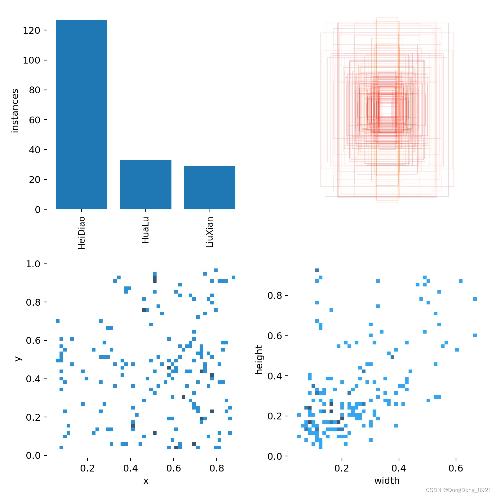
The first picture: classes (the amount of data in each category)
The second picture: labels (size and number of boxes)
The third picture: center (the coordinates of the center point of the box)
The fourth picture: labels width and height (the length and width of the box)
4.P_curve (relationship graph of accuracy and confidence)
Precision rate (precision rate): Indicates the proportion of examples that are classified as positive examples that are actually positive examples
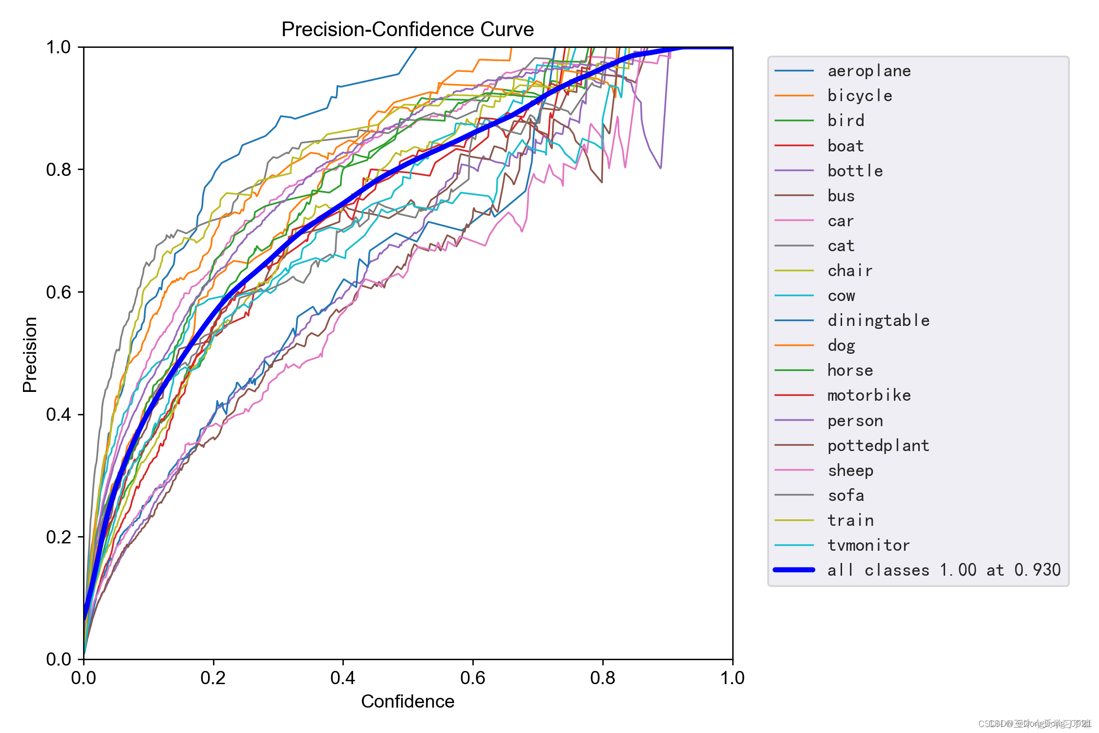
Explanation: When the confidence level is set to a certain value, the accuracy rate of each category recognition.
It can be seen that when the confidence is greater, the category detection is more accurate. This is also easy to understand. Only when the confidence level is high can it be judged to be a certain category. But in this case, some categories with low confidence will be missed.
For example, when running the program, even if a certain target is a fish, the model predicts that it is also a fish, but the confidence level given to it is only 70%. When the confidence level is set to 80%, it is considered to be a fish, and the target will be ignored.
5. R_curve (relational graph of recall and confidence)
Recall rate (recall rate): Measures that there are multiple positive examples that are classified as positive examples
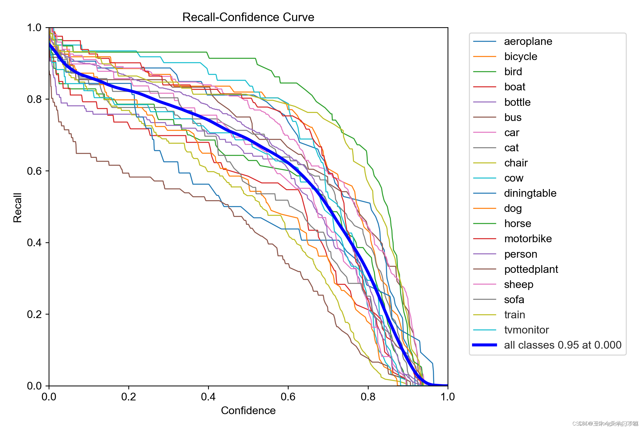
Explanation: When the confidence level is set to a certain value, the probability of recalling each category. It can be seen that when the confidence is smaller, the category detection is more comprehensive.
6. Prior knowledge synthesis recall and precision
Precision and Recall are usually a pair of contradictory performance metrics. Generally speaking, the higher the Precision, the lower the Recall.
The reason is: if we want to improve the Precision, that is, the positive examples predicted by the two classifiers are as true as possible, then we need to increase the threshold for the two classifiers to predict positive examples. For example, before predicting positive examples as long as the samples with a confidence level of 0.5 were marked as positive examples, now we need to increase the confidence level to
0.7 before we mark them as positive examples, so as to ensure that the positive examples selected by the binary classifier are more likely to be positive examples. The real positive example; and this goal is exactly the opposite of improving Recall. If we want to improve Recall, that is, the two classifiers can pick out the real positive examples as much as possible, then it is necessary to lower the threshold for the two classifiers to predict positive examples, such as the previous prediction. For example, as long as the sample with a confidence level
of 0.5 is marked as a real positive example, then if it is reduced to
0.3, we will mark it as a positive example, so as to ensure that the binary classifier selects as many as possible True example.
Note: The algorithm assigns a confidence level to each target
For the binary classifier, my understanding is: Even if there are multiple targets, because in P_curve and R_curve, each category has its own corresponding curve, so when calculating each category (such as fish), the fish is positive examples, and the rest are classified as negative examples no matter how many classes there are.
7.PR_curve (relational graph of precision rate and recall rate)
mAP (Mean Average Precision), the mean average precision.
mAP is the mean of all categories of AP, and AP is determined by precision and recall; while IoU threshold and confidence (confidence) threshold affect the calculation of precision and recall. When calculating precision and recall, it is necessary to judge TP, FP, TN, and FN
The number behind @ indicates the threshold for judging iou as a positive or negative example
It can be seen that the higher the precision, the lower the recall rate.
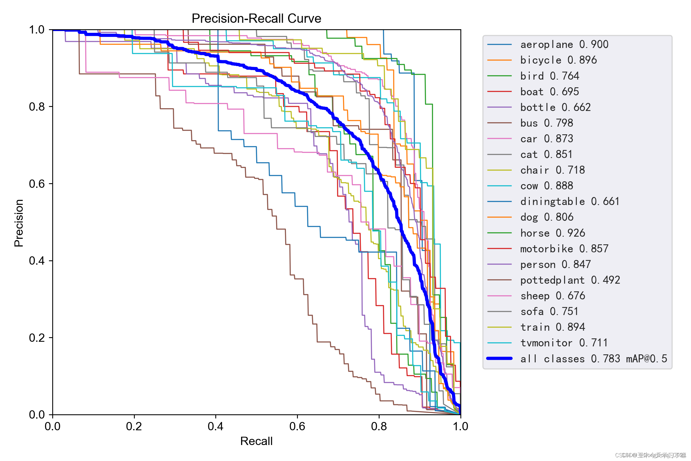
We hope that our network can detect all categories as much as possible under the premise of high accuracy. So we hope that our curve is close to the (1, 1) point, that is, we hope that the area of the mAP curve is as close to 1 as possible.
The first measure: the area of the mAP curve.
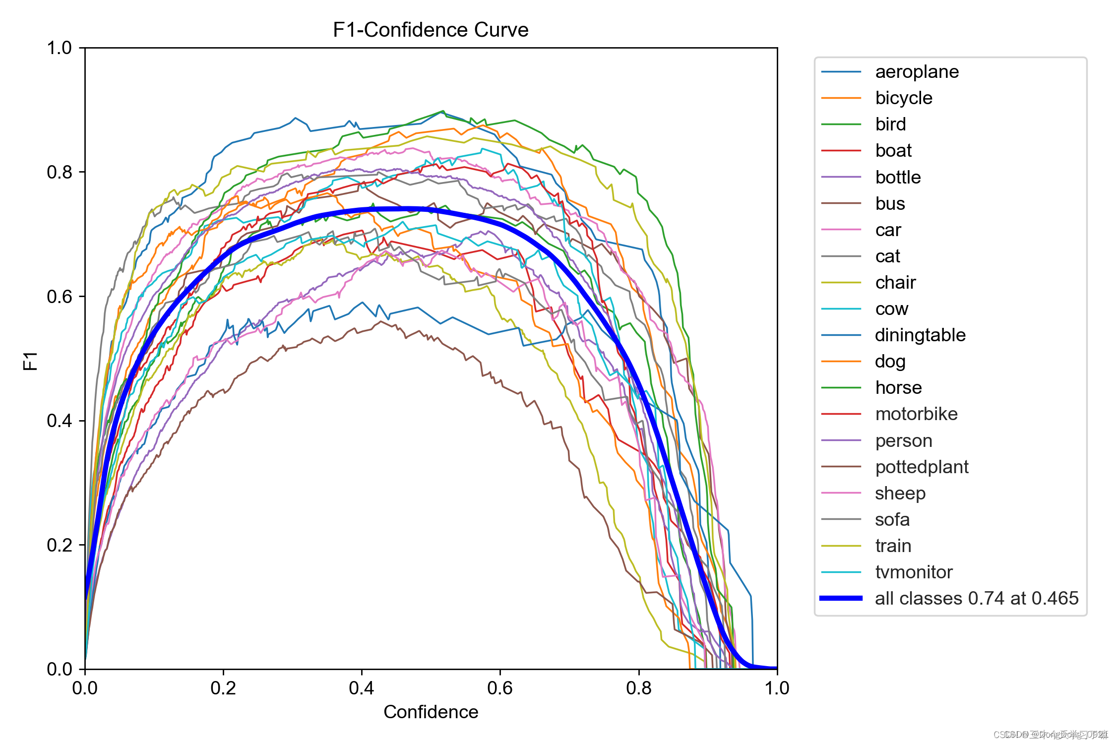
8.F1_curve
F1 score (F1-score) is a measure of classification problems. is the harmonic mean of precision and recall, with 1 being the best and 0 being the worst.
9. Analysis of visual training results
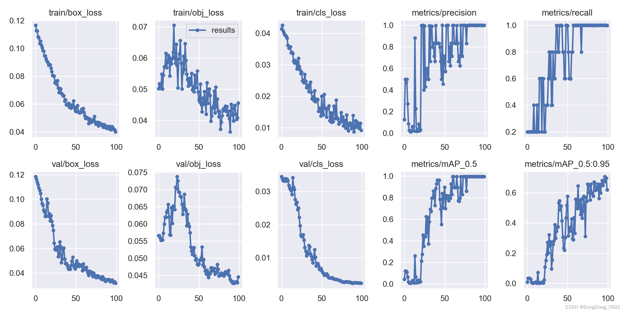
The abscissa represents the number of training rounds (epoch)
obj(Objectness): Presumably the average value of the target detection loss, the smaller the target, the more accurate the detection.
cls(Classification): Presumably the mean value of the classification loss, the smaller the classification, the more accurate it is.
The second measurement indicator: Generally speaking, the general training results mainly observe the fluctuation of precision and recall rate . If the fluctuation is not too large, the training effect is better; if the training is better, the figure shows a steady increase.
10. Small insights
Q1: In the process of learning the analysis of YOLOv5 training results, I suddenly had a question: isn't train.py just training training pictures, how can it involve the problem of accuracy?

Explanation: In the training process, one step will generate a training set (train.txt), a verification set (val.txt), and a test set (test.txt), which store the name of the picture (without the suffix .jpg).
Training set : used to train the model and determine parameters . It is equivalent to the process of teachers teaching students knowledge.
Validation set : used to determine the network structure and adjust the hyperparameters of the model . It is equivalent to a small quiz such as a monthly exam, which is used for students to check for gaps in their studies.
Test set : used to test the generalization ability of the model . It is equivalent to a big exam, like going to the battlefield, to really test the learning effect of students.
So I feel that it is in the process of testing the test set that the parameters such as precision rate and recall rate come out.
The reason why P_curve and R_curve only have black sea bream in the training result document of Bishe is that there are only pictures of black sea bream in the test set.
Here is the design of the proportion division of training set, verification set and test set (unresolved)
Semi-finished products: just to understand the specific principles of YOLOv5, if there is any infringement, please inform and delete
Category of website: technical article > Blog
Author:Disheartened
link:http://www.pythonblackhole.com/blog/article/365/923130faec3869c2aea7/
source:python black hole net
Please indicate the source for any form of reprinting. If any infringement is discovered, it will be held legally responsible.
name:
Comment content: (supports up to 255 characters)
no articles