逻辑回归(Logistic Regression)详解
posted on 2023-05-21 18:08 read(512) comment(0) like(25) collect(2)
Logistic regression, also known as logistic regression analysis, is a generalized linear regression analysis model that belongs to supervised learning in machine learning. Its derivation process and calculation method are similar to the regression process, but in fact it is mainly used to solve binary classification problems (multiple classification problems can also be solved). Train the model by given n sets of data (training set), and classify one or more sets of given data (test set) after training. Each set of data is composed of p indicators.
(1) Data processed by logistic regression
Logistic regression is used for classification. For example, we give a person's [height, weight] these two indicators, and then judge whether the person belongs to the category of "fat" or "thin". For this problem, we can first measure the height and weight of n individuals and the corresponding indicators "fat" and "thin", express fat and thin as 0 and 1 respectively, and input these n sets of data into the model for training. After training, input the height and weight of a person to be classified into the model to see whether the person is "fat" or "thin".
If the data has two indicators, the data can be represented by points on the plane, one of which is the x-axis and the other is the y-axis; if the data has three indicators, the data can be represented by points in the space; if it is p-dimensional (p>3) is a point in p-dimensional space.
Essentially, the model after logistic regression training is a straight line on the plane (p=2), or plane (p=3), hyperplane (p>3). And this line or plane divides the scattered points in the space into two halves, and most of the data belonging to the same class are distributed on the same side of the curve or plane.
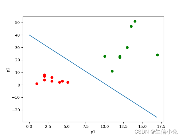
As shown in the figure above, the number of points is the number of samples, and the two colors represent two indicators. This straight line can be regarded as a straight line that divides samples after training with these samples. Then, for the values of p1 and p2 of the subsequent samples, you can judge which category it belongs to according to this straight line.
(2) Algorithm principle
First, we deal with binary classification problems. Since it is divided into two categories, we let one of the labels be 0 and the other one is 1. We need a function that can be mapped to a number between 0 and 1 for each set of input data . And if the function value is greater than 0.5, it is determined to belong to 1, otherwise it belongs to 0. Moreover, the function needs to be undetermined parameters. By using sample training, this parameter can be accurately predicted for the data in the training set.
This function is the sigmoid function, of the form . So here we can set the function as
Here is the i-th data of the test set, which is a p-dimensional column vector
; w is a p-dimensional column vector
, which is the parameter to be requested; b is a number, which is also the parameter to be requested.
We found that, for , the result was
. So we can put
w written ,
written
.
can be written
as:
This allows another parameter b to be incorporated into w . It is also much more convenient to deduce later. Of course, we can also use the first form to do it, the essence is the same. After that, the parameter w is calculated according to the training samples.
(3) Solve the parameters.
This part is the core problem of logistic regression. Tutu will give two methods below.
(1) Maximum likelihood estimation.
Maximum likelihood estimation is an important method of parameter estimation in mathematical statistics. The idea is that when an event happens, the probability of this event happening is the greatest. For sample i, its category is . For sample i, it can be
regarded as a probability. When yi corresponds to 1, the probability is h(xi), that is, the possibility that xi belongs to 1; when yi corresponds to 0, the probability is 1-h(xi), that is, the possibility that xi belongs to 0. Then it constructs the maximum likelihood function
.
Among them, i from 0 to k is the number k belonging to category 1, and i from k+1 to n is the number nk belonging to category 0. Since y is the label 0 or 1, the above formula can also be written as:
In this way, no matter whether y is 0 or 1, one of them will always become the power of 0, that is, 1, which is equivalent to the first formula.
For convenience, we take the logarithm of the expression. Because it is to find the maximum value of the formula, it can be converted into the formula multiplied by negative 1, and then find the minimum value. At the same time, for n pieces of data, the value after accumulation will be very large, and if gradient descent is used later, it will easily lead to gradient explosion. So it can be divided by the total number of samples n.
There are many ways to find the minimum value, and the gradient descent series method is commonly used in machine learning. Newton's method can also be used, or the value of w when the derivative is zero, etc.
(2) Loss function
The cross-entropy loss function is commonly used in logistic regression, and the cross-entropy loss function is the same as the loss function obtained by the maximum likelihood method above. I won't go into details here. The other can also use the square loss function (mean square error), that is
This is relatively intuitive. It is to make this prediction function h(xi) as close as possible to the actual classification 1 or 0. That is, the smaller the loss function, the better. Finding the minimum value still uses the method mentioned above.
So far we have got these two functions here. Let's take gradient descent as an example, which is to find the derivative of the loss function.
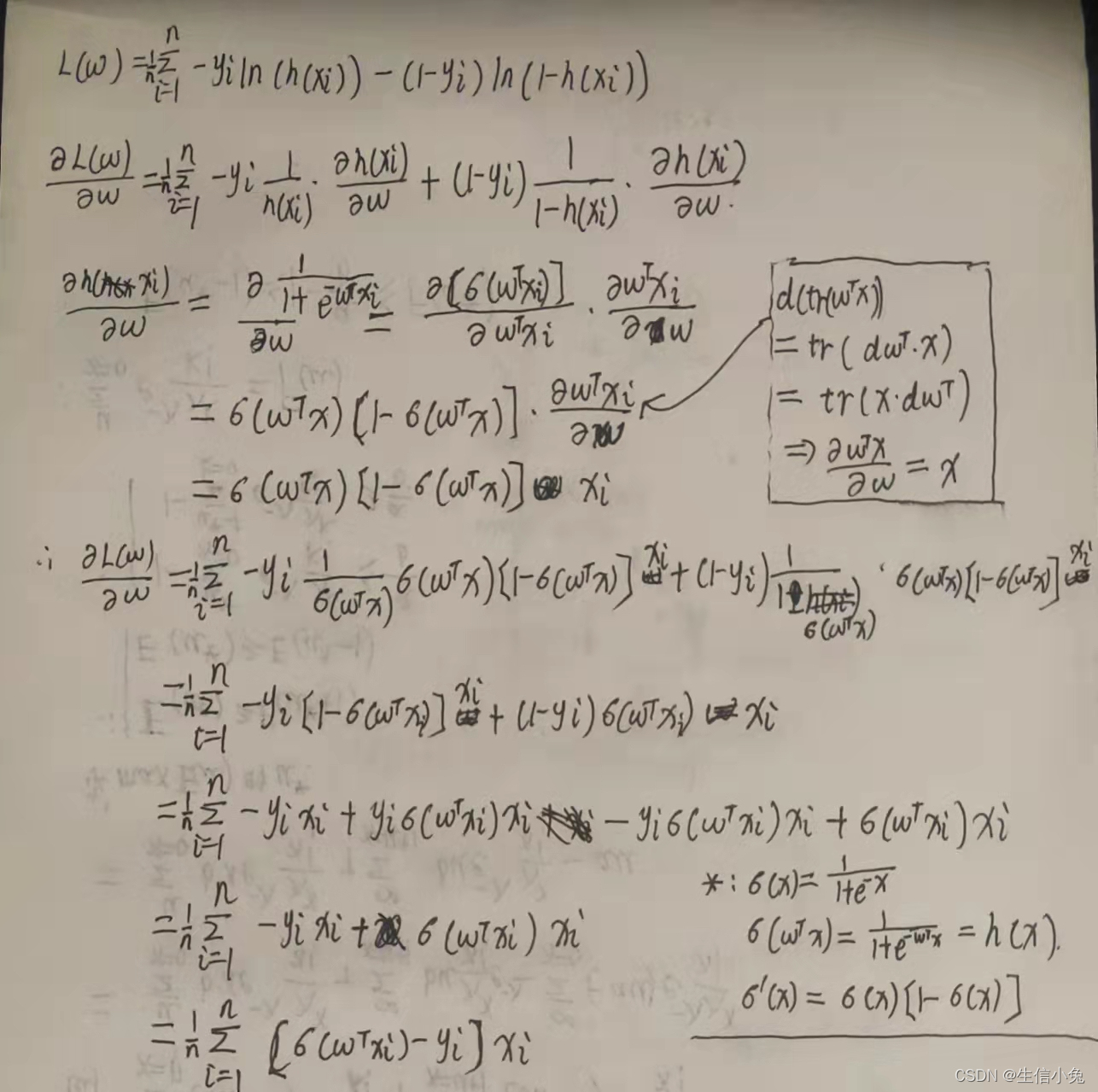
For the loss function (1), the derivative solution process is as follows (matrix derivation is required).
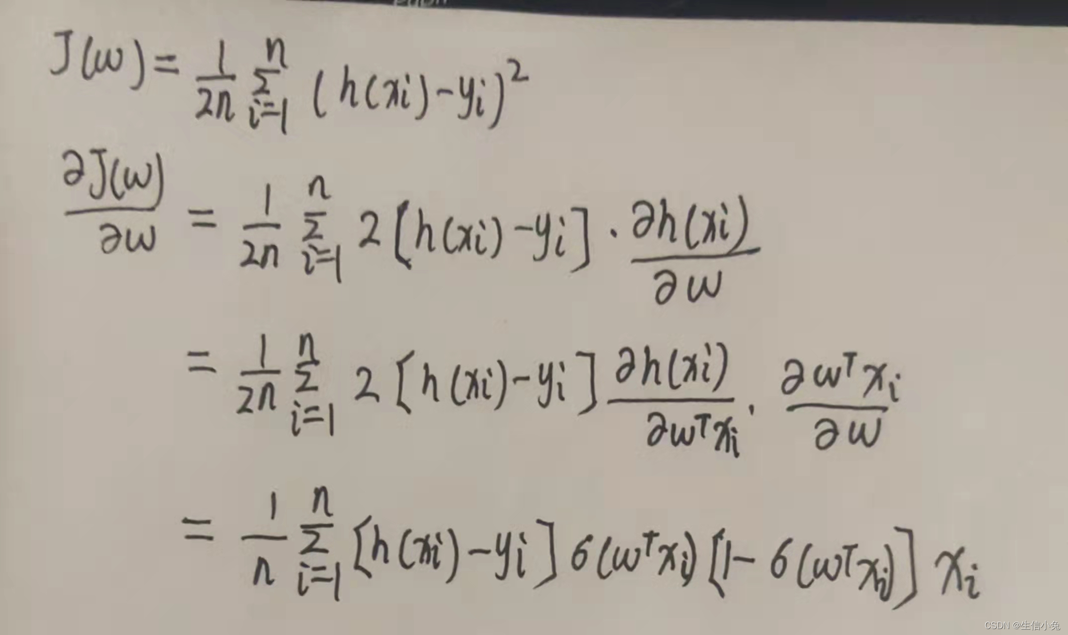
For the loss function (2), the derivation process is as follows:
(3) Algorithm implementation.
Tutu takes the Dry_Bean_Dataset file as an example here. Students can download the data set from www.kaggle.com, which should be more convenient.
- import pandas as pd
- data=pd.read_csv('Dry_Bean_Dataset.csv')
- df=pd.DataFrame(data)
- print(df.columns,df.shape)
Let's take a look at the data set first. There are many indicators in it, including the area of the bean, the circumference, the length of the major axis, and the length of the minor axis. class represents the type of the corresponding bean. For the sake of intuition and convenience (easy to express on a two-dimensional plane), we choose the two indicators of MajorAxisLength and MinorAxisLength. Since it is a binary classification, we choose the two categories SEKER and BARBUNYA, that is, the first 3349 sets of data. Draw a scatterplot of observations.
- import pandas as pd
- import matplotlib.pyplot as plt
- data=pd.read_csv('Dry_Bean_Dataset.csv')
- df=pd.DataFrame(data)
- color=[]
- for i in df['Class'][0:3349]:
- if i=='SEKER':
- color.append('red')
- else:
- color.append('blue')
- plt.scatter(df['MajorAxisLength'][0:3349],df['MinorAxisLength'][0:3349],color=color)
- plt.xlabel('MajorAxisLength')
- plt.ylabel('MinorAxisLength')
- plt.show()
The scatterplot is as follows:
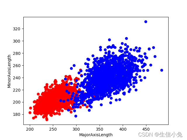
It can be seen that the data can be divided into two parts by a straight line.
After that, we need to process the data a bit. Bind the two indicators of each set of data and their corresponding classifications (if stochastic gradient descent needs to be handled like this, batch gradient descent can not be handled this way), and convert each set of data into a column vector.
- import numpy as np
- import pandas as pd
- data=pd.read_csv('Dry_Bean_Dataset.csv')
- df=pd.DataFrame(data)
- label=[]
- for i in df['Class'][0:3349]:
- if i=='SEKER':
- label.append(0)
- else:
- label.append(1)
- x1=df['MajorAxisLength'][0:3349]
- x2=df['MinorAxisLength'][0:3349]
- train_data=list(zip(x1,x2,label))
- class Logistic_Regression:
- def __init__(self,traindata,alpha=0.001,circle=1000,batchlength=40):
- self.traindata=traindata #训练数据集
- self.alpha=alpha #学习率
- self.circle=circle #学习次数
- self.batchlength=batchlength #把3349个数据分成多个部分,每个部分有batchlength个数据
- self.w=np.random.normal(size=(3,1)) #随机初始化参数w
- def data_process(self):
- '''做随机梯度下降,打乱数据顺序,并把所有数据分成若干个batch'''
- np.random.shuffle(self.traindata)
- data=[self.traindata[i:i+self.batchlength]
- for i in range(0,len(self.traindata),self.batchlength)]
- return data
- def train1(self):
- '''根据损失函数(1)来进行梯度下降,这里采用随机梯度下降'''
- for i in range(self.circle):
- batches=self.data_process()
- print('the {} epoch'.format(i)) #程序运行时显示执行次数
- for batch in batches:
- d_w=np.zeros(shape=(3,1)) #用来累计w导数值
- for j in batch: #取batch中每一组数据
- x0=np.r_[j[0:2],1] #把数据中指标取出,后面补1
- x=np.mat(x0).T #转化成列向量
- y=j[2] #标签
- dw=(self.sigmoid(self.w.T*x)-y)[0,0]*x
- d_w+=dw
- self.w-=self.alpha*d_w/self.batchlength
-
- def train2(self):
- '''用均方损失函数来进行梯度下降求解'''
- for i in range(self.circle):
- batches=self.data_process()
- print('the {} epoch'.format(i)) #程序运行时显示执行次数
- for batch in batches:
- d_w=np.zeros(shape=(3,1)) #用来累计w导数值
- for j in batch: #取batch中每一组数据
- x0=np.r_[j[0:2],1] #把数据中指标取出,后面补1
- x=np.mat(x0).T #转化成列向量
- y=j[2] #标签
- dw=((self.sigmoid(self.w.T*x)-y)*self.sigmoid(self.w.T*x)*(1-self.sigmoid(self.w.T*x)))[0,0]*x
- d_w+=dw
- self.w-=self.alpha*d_w/self.batchlength
-
- def sigmoid(self,x):
- return 1/(1+np.exp(-x))
-
- def predict(self,x):
- '''测试新数据属于哪一类,x是2维列向量'''
- s=self.sigmoid(self.w.T*x)
- if s>=0.5:
- return 1
- elif s<0.5:
- return 0
- if __name__=='__main__':
- regr=Logistic_Regression(traindata=train_data)
- regr.train1() #采用1的方式进行训练

The processing needs to pay attention to the type of data. For example, when the row vector and the column vector are multiplied into a number, we calculate a number, but numpy returns a 1x1 matrix, so it will be wrong to multiply it with the following vector, so we need to pay attention to converting the matrix into a number.
So, how to observe the effect more intuitively for this model? We know that in the end x is substituted into h( x ), the closer the value is to 1, the more likely it belongs to category 1, and the closer to 0, the more likely it belongs to category 0; then when h( x ) =0.5, x is above the dividing line at this time up. So from , it finally follows that
, ie
. This is the equation of the dividing line.
- w=regr.w
- w1=w[0,0]
- w2=w[1,0]
- w3=w[2,0]
- x=np.arange(190,500)
- y=-w1*x/w2-w3/w2
- plt.plot(x,y)
- plt.show()
In order to dynamically observe the straight line transformation, this part can also be placed in the train() function.
For the above running results, we can find that the effect is not very good. On the one hand, the running speed is very slow, and a slightly larger alpha setting can easily cause overflow under the sigmoid function. On the other hand, we found that the straight line did not completely separate the two sets of data, and even passed through two areas.
Regarding this phenomenon, Tutu believes that: the number of data sets is large, and each time the data is processed, a large amount of calculation is required, resulting in slow running speed. The solution is: each circle can only randomly select part of the data for training; for the function The phenomenon of overflow is that it becomes a very small negative number during the running process, resulting in too large exponential operation, so the learning rate can be reduced to prevent w from becoming a
very small value after one iteration; the straight line does not completely divide the two parts , we can consider it from the aspect of data characteristics, because we artificially select two indicators at random, and then train and judge the classification standard according to these two indicators, it is easy to have problems in this way, we do not know the data characteristics of the two indicators It is not clear whether other indicators play a decisive role in the classification, and the two types of data have many common parts overlapping, which also leads to problems in classification. When we finished the training, we found that although the straight line passes through the two regions, it is a straight line with a positive slope, but in fact it also divides the core part of the two regions (the most concentrated part of the two types of data) into two parts, indicating that This part of the data plays a major role, and the ultimate goal of logistic regression training is to minimize the loss function, indicating that the final curve also meets the requirements.
In order to intuitively reflect the training characteristics of logistic regression, Tutu selected a part of the iris data set for training, and the effect is shown in the figure below.
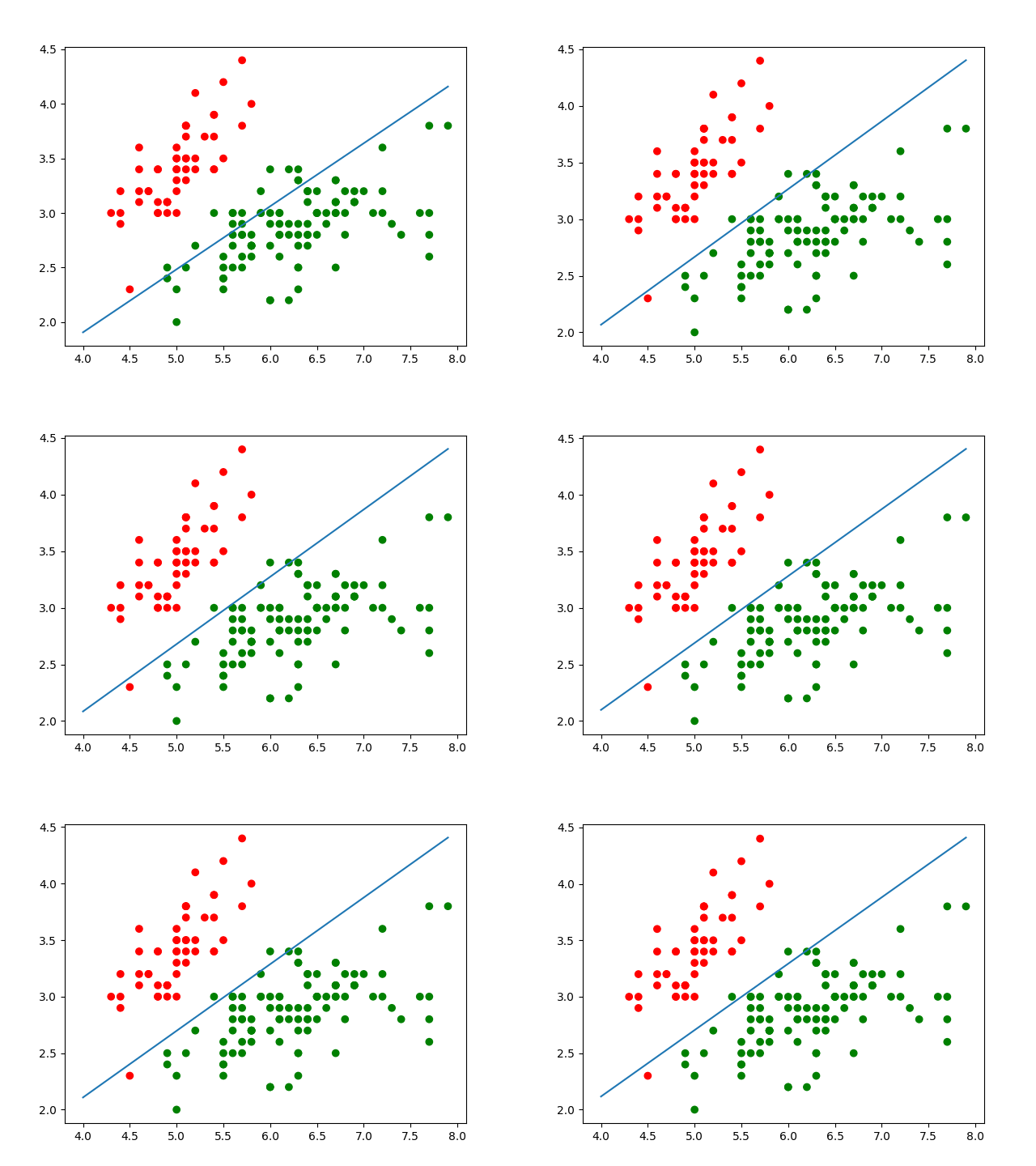
In the case above, it basically stabilizes near the optimal solution after dozens of cycles. If the learning rate and other parameters are not properly adjusted, the following situations may occur:
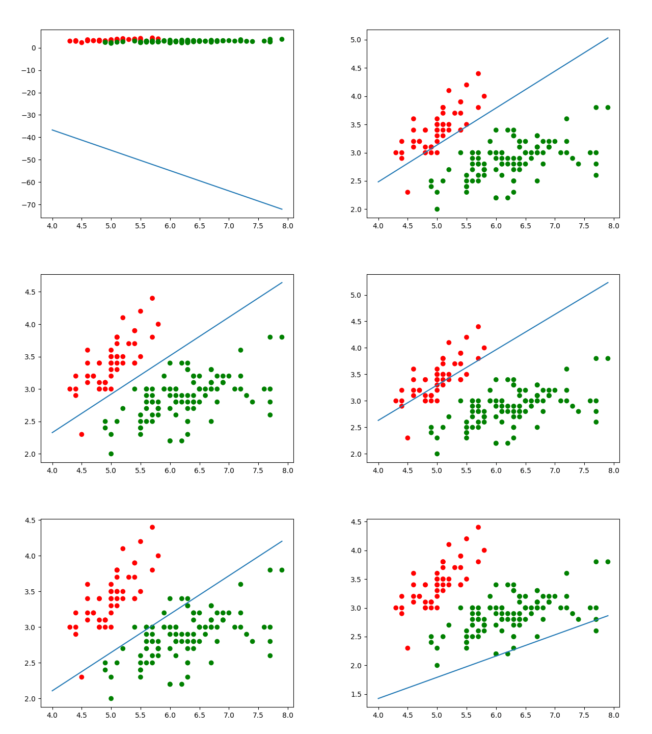
(4) Nonlinear logistic regression
Nonlinear logistic regression should be more commonly used than linear logistic regression. For example, when two sets of data cannot be divided by a straight line or a plane, but need a curve or a curved surface to be divided. At this time, nonlinear logistic regression can be used. For example, use a circle, ellipse, curve, etc. to separate two sets of data.
The training and derivation process of nonlinear regression is the same as the previous one. Just deal with the two indicators of x1 and x2. This process is consistent with the nonlinear regression that Tutu mentioned before (for details, see: "Linear Regression (Linear Fitting) and Nonlinear Regression (Nonlinear Fitting) Principles, Derivation and Algorithm Implementation (1)").
We found earlier that the curve equation we finally trained is . Then, if we make , the vector x
of each set of inputs is processed into: , which is similar to polynomial regression. In this way, after training, the area can be segmented with a curve equation in the form of this. The same is true for three-dimensional and p-dimensional. We can even adjust the degree of polynomial, or the form of the function, etc. as needed, so as to achieve the desired effect. But at this time, we should pay attention to the occurrence of over-fitting and under-fitting , and regularization and other processing methods are needed.
(5) Multi-classification problems of logistic regression.
What I said above is the binary classification problem of logistic regression, so can logistic regression handle multi-classification? The answer is yes. At this time we no longer use the sigmoid function, but another function called softmax. The function form is as follows:
Then the h(x) function is
Here again, we represent the k classes with numbers 1, 2...k, and in the sigmoid function, the function value represents the probability. The same is true here, after x is processed by the h function, the value of the corresponding position (category) in the vector obtained is the probability of taking the corresponding position (category). For example, for a three-category problem, if p(y=1)=0.7, p(y=2)=0.2, p(y=3)=0.1 in the vector, then the probability of x belonging to class 1 is the largest, so the discrimination is 1 kind.
Its derivation process is similar to the previous one. It also constructs the loss function, finds the derivative of the loss function with respect to w , and performs gradient descent processing calculations.
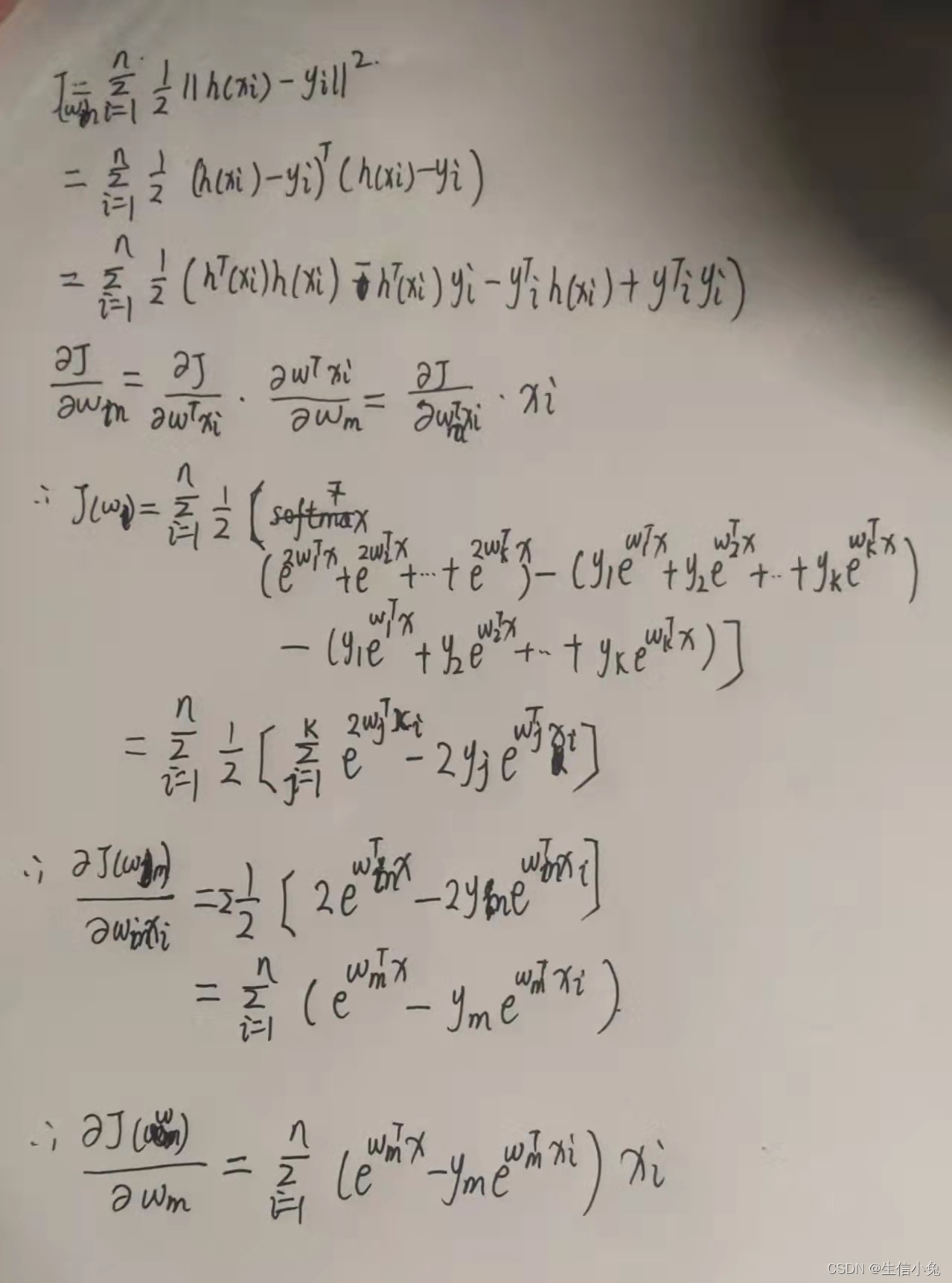
The mean square loss is used here. The derivation process is as shown above. Partial derivatives are obtained for each w, and then the corresponding w can be used for gradient descent.
(6) Summary.
Logistic regression can be divided into linear and nonlinear, and can also be divided into binary classification and multi-classification problems according to the number of classes. It needs to be used flexibly when used. It can construct loss functions and find gradients. At the same time, it can be implemented by algorithms and trained for prediction.
In fact, careful students will find that in logistic regression, we find that there are multiple inputs (that is, p indicators), and finally output a result (0 or 1). The process is to multiply the input by weight w plus bias b ( In this paper, the weight w and bias b are merged into w), and then the result is processed by the sigmoid function. This process is actually very close to the neural network, and the logistic regression model is closer to the perceptron. For the neural network, it not only has two layers of input and output, but also adds more hidden layers, and the processing results of each layer are used as the input of the next layer, so the solution of its loss function and gradient will also be more complicated. The model is also much more complex.
Category of website: technical article > Blog
Author:gfg
link:http://www.pythonblackhole.com/blog/article/25313/533fe88d1afdd1a24992/
source:python black hole net
Please indicate the source for any form of reprinting. If any infringement is discovered, it will be held legally responsible.
name:
Comment content: (supports up to 255 characters)
no articles