Simple implementation of GCN-graph convolutional neural network algorithm (including python code)
posted on 2023-05-21 17:21 read(1120) comment(0) like(22) collect(2)
This article is an introduction to the code for implementing the GCN algorithm model. The previous article is an introduction to the principle and model of the GCN algorithm.
The Cora dataset used in the code:
Link: https://pan.baidu.com/s/1SbqIOtysKqHKZ7C50DM_eA
Extraction code: pfny
Article directory
2. Explanation of the realization process
3. Code implementation and result analysis
3. Definition of graph convolution layer
4. GCN graph convolutional neural network model definition
5.1 Definition of hyperparameters, including learning rate, regularization coefficient, etc.
5.3 Define training and test functions, and perform training
Purpose
The purpose of this experiment is to classify the papers, through model training, use the training set that has been classified, and divide the papers into 7 categories through the GCN algorithm.
1. Dataset introduction
The data set I choose is the Cora data set commonly used by GCN. The goal of the experiment is to classify the sample nodes of the data set by training the constructed two-layer GCN model.
Cora dataset download address: https://linqs-data.soe.ucsc.edu/public/lbc/cora.tgz
Personally, I don't recommend using the Cora data in python's dgl package, it always reports an error.
The Cora dataset consists of papers on machine learning. These papers fall into one of seven categories:
1. Case-based
2. Genetic algorithm
3. Neural network
4. Probabilistic methods
5. Reinforcement Learning
6. Rule learning
7. Theory
The papers were screened such that each paper cited or was cited by at least one other paper in the final dataset. There are 2708 papers in the entire corpus.
After stemming and removing endings, only 1433 unique words remained. All words with a document frequency less than 10 are removed.
That is, the Cora dataset contains 2708 vertices, 5429 edges, each vertex contains 1433 features, and there are 7 categories in total.
And Cora has already divided the data of the training set and the test set, just read the data directly according to the file name, such as
File ind.cora.x => feature vector of training instance; ind.cora.y => label of training instance, one-hot encoding
ind.cora.tx => feature vector of test instance; ind.cora.ty => label of test instance, one-hot encoding
2. Explanation of the realization process
Combined with the code implementation I made last, I will give you a simple example of the citation network, so that you can understand the processing process.
Each node represents a research paper, while an edge represents a citation relationship.
We have a preprocessing step here. Here we don't use original papers as features, but convert papers into vectors (by using NLP embeddings such as tf-idf).
Suppose we use the average() function (in fact, the internal transfer function of GCN is definitely not the average value, this is just for easy understanding). We will do the same for all nodes to get the feature vector. Finally, we feed these calculated averages into the neural network.
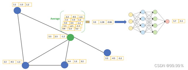
Let's consider the green nodes. First, we get the eigenvalues of all its neighbors, including itself, and take the average. Finally, a result vector is returned through the neural network and used as the final result. Note that in GCN, we only use one fully connected layer. In this example, we get 2D vector as output (2 nodes of fully connected layer).
The function of the fully connected network is to multiply the vector obtained by the previous layer, and finally reduce its dimension, and then input it into the softmax layer to obtain the corresponding score of each category.
In actual operation, we must use a more complex aggregation function than the average function, which is the propagation function mentioned above.
We can also stack more layers together to get a deeper GCN. The output of each layer is considered as the input of the next layer.
Example of 2-layer GCN: the output of the first layer is the input of the second layer.
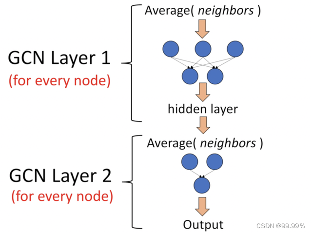
Then the two-layer GCN can obtain the characteristics of the second-order neighbor nodes through the formula of inter-layer propagation while reducing the dimension:
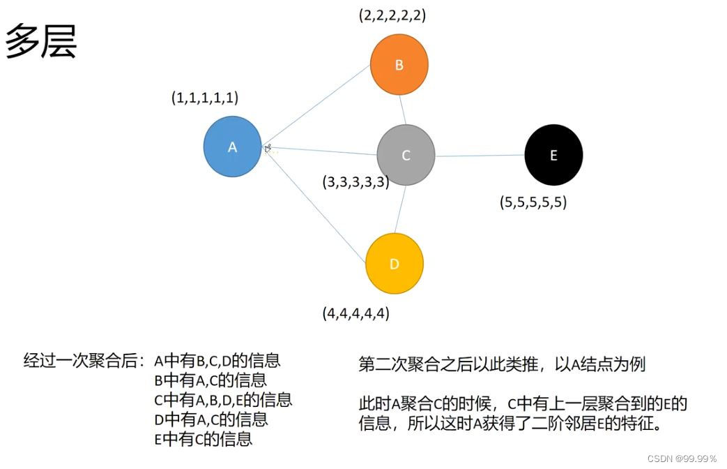
In the node classification problem, in fact, the input adjacency matrix and the characteristics of each node include both the connection between nodes and the characteristics of the node itself.
Dimensionality reduction can be achieved through the convolutional layer of GCN, and if you want to cluster into several categories, you can reduce it to a few dimensions.
3. Code implementation and result analysis
1. Import package
- import itertools
- import os
- import os.path as osp
- import pickle
- import urllib
- from collections import namedtuple
- import warnings
- warnings.filterwarnings("ignore")
- import numpy as np
- import scipy.sparse as sp
- import torch
- import torch.nn as nn
- import torch.nn.functional as F
- import torch.nn.init as init
- import torch.optim as optim
- import matplotlib.pyplot as plt
- %matplotlib inline

2. Data preparation
- Data = namedtuple('Data', ['x', 'y', 'adjacency',
- 'train_mask', 'val_mask', 'test_mask'])
-
-
- def tensor_from_numpy(x, device):
- return torch.from_numpy(x).to(device)
-
-
- class CoraData(object):
- filenames = ["ind.cora.{}".format(name) for name in
- ['x', 'tx', 'allx', 'y', 'ty', 'ally', 'graph', 'test.index']]
-
- def __init__(self, data_root="./data", rebuild=False):
- """Cora数据,包括数据下载,处理,加载等功能
- 当数据的缓存文件存在时,将使用缓存文件,否则将下载、进行处理,并缓存到磁盘
- 处理之后的数据可以通过属性 .data 获得,它将返回一个数据对象,包括如下几部分:
- * x: 节点的特征,维度为 2708 * 1433,类型为 np.ndarray
- * y: 节点的标签,总共包括7个类别,类型为 np.ndarray
- * adjacency: 邻接矩阵,维度为 2708 * 2708,类型为 scipy.sparse.coo.coo_matrix
- * train_mask: 训练集掩码向量,维度为 2708,当节点属于训练集时,相应位置为True,否则False
- * val_mask: 验证集掩码向量,维度为 2708,当节点属于验证集时,相应位置为True,否则False
- * test_mask: 测试集掩码向量,维度为 2708,当节点属于测试集时,相应位置为True,否则False
- Args:
- -------
- data_root: string, optional
- 存放数据的目录,原始数据路径: ../data/cora
- 缓存数据路径: {data_root}/ch5_cached.pkl
- rebuild: boolean, optional
- 是否需要重新构建数据集,当设为True时,如果存在缓存数据也会重建数据
- """
- self.data_root = data_root #数据存放的路径
- save_file = osp.join(self.data_root, "ch5_cached.pkl")
- if osp.exists(save_file) and not rebuild:
- print("Using Cached file: {}".format(save_file))
- self._data = pickle.load(open(save_file, "rb"))
- else:
- self._data = self.process_data()
- with open(save_file, "wb") as f:
- pickle.dump(self.data, f)
- print("Cached file: {}".format(save_file))
-
- @property
- def data(self):
- """返回Data数据对象,包括x, y, adjacency, train_mask, val_mask, test_mask"""
- return self._data
-
- def process_data(self):
- """
- 处理数据,得到节点特征和标签,邻接矩阵,训练集、验证集以及测试集
- 引用自:https://github.com/rusty1s/pytorch_geometric
- """
- print("Process data ...")
- _, tx, allx, y, ty, ally, graph, test_index = [self.read_data(
- osp.join(self.data_root, name)) for name in self.filenames]
- train_index = np.arange(y.shape[0])
- val_index = np.arange(y.shape[0], y.shape[0] + 500)
- sorted_test_index = sorted(test_index)
-
- x = np.concatenate((allx, tx), axis=0) #节点特征
- y = np.concatenate((ally, ty), axis=0).argmax(axis=1) #标签
-
- x[test_index] = x[sorted_test_index]
- y[test_index] = y[sorted_test_index]
- num_nodes = x.shape[0]
-
- train_mask = np.zeros(num_nodes, dtype=np.bool) #训练集
- val_mask = np.zeros(num_nodes, dtype=np.bool) #验证集
- test_mask = np.zeros(num_nodes, dtype=np.bool) #测试集
- train_mask[train_index] = True
- val_mask[val_index] = True
- test_mask[test_index] = True
-
-
- """"构建邻接矩阵"""
- adjacency = self.build_adjacency(graph)
- print("Node's feature shape: ", x.shape)
- print("Node's label shape: ", y.shape)
- print("Adjacency's shape: ", adjacency.shape)
- print("Number of training nodes: ", train_mask.sum())
- print("Number of validation nodes: ", val_mask.sum())
- print("Number of test nodes: ", test_mask.sum())
-
- return Data(x=x, y=y, adjacency=adjacency,
- train_mask=train_mask, val_mask=val_mask, test_mask=test_mask)
-
- @staticmethod
- def build_adjacency(adj_dict):
- """根据邻接表创建邻接矩阵"""
- edge_index = []
- num_nodes = len(adj_dict)
- for src, dst in adj_dict.items():
- edge_index.extend([src, v] for v in dst)
- edge_index.extend([v, src] for v in dst)
- # 去除重复的边
- edge_index = list(k for k, _ in itertools.groupby(sorted(edge_index)))
- edge_index = np.asarray(edge_index)
- adjacency = sp.coo_matrix((np.ones(len(edge_index)),
- (edge_index[:, 0], edge_index[:, 1])),
- shape=(num_nodes, num_nodes), dtype="float32")
- return adjacency
-
- @staticmethod
- def read_data(path):
- """使用不同的方式读取原始数据以进一步处理"""
- name = osp.basename(path)
- if name == "ind.cora.test.index":
- out = np.genfromtxt(path, dtype="int64")
- return out
- else:
- out = pickle.load(open(path, "rb"), encoding="latin1")
- out = out.toarray() if hasattr(out, "toarray") else out
- return out
-
- @staticmethod
- def normalization(adjacency):
- """计算 H=D^-0.5 * (A+I) * D^-0.5"""
- adjacency += sp.eye(adjacency.shape[0]) # 增加自连接
- degree = np.array(adjacency.sum(1))
- d_hat = sp.diags(np.power(degree, -0.5).flatten())
- return d_hat.dot(adjacency).dot(d_hat).tocoo()

3. Definition of graph convolution layer
- class GraphConvolution(nn.Module):
- def __init__(self, input_dim, output_dim, use_bias=True):
- """图卷积:H*X*\theta
- Args:
- ----------
- input_dim: int
- 节点输入特征的维度
- output_dim: int
- 输出特征维度
- use_bias : bool, optional
- 是否使用偏置
- """
- super(GraphConvolution, self).__init__()
- self.input_dim = input_dim
- self.output_dim = output_dim
- self.use_bias = use_bias
- self.weight = nn.Parameter(torch.Tensor(input_dim, output_dim))
- if self.use_bias:
- self.bias = nn.Parameter(torch.Tensor(output_dim))
- else:
- self.register_parameter('bias', None)
- self.reset_parameters() #初始化w
-
- def reset_parameters(self):
- init.kaiming_uniform_(self.weight)
- #init.kaiming_uniform_神经网络权重初始化,神经网络要优化一个非常复杂的非线性模型,而且基本没有全局最优解,
- #初始化在其中扮演着非常重要的作用,尤其在没有BN等技术的早期,它直接影响模型能否收敛。
-
- if self.use_bias:
- init.zeros_(self.bias)
-
- def forward(self, adjacency, input_feature):
- """邻接矩阵是稀疏矩阵,因此在计算时使用稀疏矩阵乘法
-
- Args:
- -------
- adjacency: torch.sparse.FloatTensor
- 邻接矩阵
- input_feature: torch.Tensor
- 输入特征
- """
- support = torch.mm(input_feature, self.weight)
- output = torch.sparse.mm(adjacency, support)
- if self.use_bias:
- output += self.bias
- return output
-
- def __repr__(self):
- return self.__class__.__name__ + ' (' \
- + str(self.input_dim) + ' -> ' \
- + str(self.output_dim) + ')'

4. GCN graph convolutional neural network model definition
With the data and the GCN layer, the model can be built for training.
Define a two-layer GCN, where the input dimension is 1433, the hidden layer dimension is set to 16, and the last layer of GCN changes the output dimension to 7 categories, and the activation function uses ReLU.
- class GcnNet(nn.Module):
- """
- 定义一个包含两层GraphConvolution的模型
- """
- def __init__(self, input_dim=1433):
- super(GcnNet, self).__init__()
- self.gcn1 = GraphConvolution(input_dim, 16)
- self.gcn2 = GraphConvolution(16, 7)
-
- def forward(self, adjacency, feature):
- h = F.relu(self.gcn1(adjacency, feature))
- logits = self.gcn2(adjacency, h)
- return logits
5. Model Training
5.1 Definition of hyperparameters, including learning rate, regularization coefficient, etc.
- LEARNING_RATE = 0.1 #学习率 学习率过小→ →→收敛过慢,学习率过大→ →→错过局部最优;
- WEIGHT_DACAY = 5e-4 #正则化系数 weight_dacay,解决过拟合问题
- EPOCHS = 200 #完整遍历训练集的次数
- DEVICE = "cuda" if torch.cuda.is_available() else "cpu" #指定设备,如果当前显卡忙于其他工作,可以设置为 DEVICE = "cpu",使用cpu运行
Why do we need to train for 200 rounds, because we don't know the weight of the edge at the beginning, and we need to train the appropriate weight through the model, which is W in the formula.
- # 加载数据,并转换为torch.Tensor
- dataset = CoraData().data
- node_feature = dataset.x / dataset.x.sum(1, keepdims=True) # 归一化数据,使得每一行和为1
- tensor_x = tensor_from_numpy(node_feature, DEVICE)
- tensor_y = tensor_from_numpy(dataset.y, DEVICE)
- tensor_train_mask = tensor_from_numpy(dataset.train_mask, DEVICE)
- tensor_val_mask = tensor_from_numpy(dataset.val_mask, DEVICE)
- tensor_test_mask = tensor_from_numpy(dataset.test_mask, DEVICE)
- normalize_adjacency = CoraData.normalization(dataset.adjacency) # 规范化邻接矩阵
-
- num_nodes, input_dim = node_feature.shape
- indices = torch.from_numpy(np.asarray([normalize_adjacency.row,
- normalize_adjacency.col]).astype('int64')).long()
- values = torch.from_numpy(normalize_adjacency.data.astype(np.float32))
- tensor_adjacency = torch.sparse.FloatTensor(indices, values,
- (num_nodes, num_nodes)).to(DEVICE)

5.2 Define the model:
- # 模型定义:Model, Loss, Optimizer
- model = GcnNet(input_dim).to(DEVICE)
- criterion = nn.CrossEntropyLoss().to(DEVICE) #nn.CrossEntropyLoss()函数计算交叉熵损失
- optimizer = optim.Adam(model.parameters(),
- lr=LEARNING_RATE,
- weight_decay=WEIGHT_DACAY)
When defining the model, the criterion is also conveniently defined, that is, the cross-entropy loss can be calculated with the nn.CrossEntropyLoss() function during the training process:

5.3 Define training and test functions, and perform training
- # 训练主体函数
- def train():
- loss_history = []
- val_acc_history = []
- model.train()
- train_y = tensor_y[tensor_train_mask]
-
- for epoch in range(EPOCHS):
- # 共进行200次训练
- logits = model(tensor_adjacency, tensor_x) # 前向传播
- #其中logits是模型输出,tensor_adjacency, tensor_x分别是邻接矩阵和节点特征。
-
- train_mask_logits = logits[tensor_train_mask] # 只选择训练节点进行监督
- loss = criterion(train_mask_logits, train_y) # 计算损失值,目的是优化模型,获得更科学的权重W
- optimizer.zero_grad()
- loss.backward() # 反向传播计算参数的梯度
- optimizer.step() # 使用优化方法进行梯度更新
- train_acc, _, _ = test(tensor_train_mask) # 计算当前模型训练集上的准确率
- val_acc, _, _ = test(tensor_val_mask) # 计算当前模型在验证集上的准确率
-
- # 记录训练过程中损失值和准确率的变化,用于画图
- loss_history.append(loss.item())
- val_acc_history.append(val_acc.item())
- print("Epoch {:03d}: Loss {:.4f}, TrainAcc {:.4}, ValAcc {:.4f}".format(
- epoch, loss.item(), train_acc.item(), val_acc.item()))
-
- return loss_history, val_acc_history
-
-
- # 测试函数
- def test(mask):
- model.eval() # 表示将模型转变为evaluation(测试)模式,这样就可以排除BN和Dropout对测试的干扰
-
- with torch.no_grad(): # 显著减少显存占用
- logits = model(tensor_adjacency, tensor_x) #(N,16)->(N,7) N节点数
- test_mask_logits = logits[mask] # 矩阵形状和mask一样
-
- predict_y = test_mask_logits.max(1)[1] # 返回每一行的最大值中索引(返回最大元素在各行的列索引)
- accuarcy = torch.eq(predict_y, tensor_y[mask]).float().mean()
- return accuarcy, test_mask_logits.cpu().numpy(), tensor_y[mask].cpu().numpy()

Use the above code for model training, you can see the log output as shown in the following code:
- loss, val_acc = train()
- test_acc, test_logits, test_label = test(tensor_test_mask)
- print("Test accuarcy: ", test_acc.item())#item()返回的是一个浮点型数据,测试集准确率
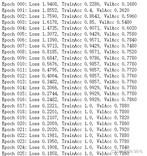
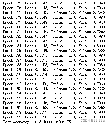
Where Epoch is the number of training rounds; loss is the loss value; the accuracy of the TrainAcc training set; the accuracy of the ValAcc test set;
6. Visualization
Visualize trends in loss and validation accuracy:
The loss function is used to measure the difference between the output value of the model and the true dependent variable value
- def plot_loss_with_acc(loss_history, val_acc_history):
- fig = plt.figure()
- # 坐标系ax1画曲线1
- ax1 = fig.add_subplot(111) # 指的是将plot界面分成1行1列,此子图占据从左到右从上到下的1位置
- ax1.plot(range(len(loss_history)), loss_history,
- c=np.array([255, 71, 90]) / 255.) # c为颜色
- plt.ylabel('Loss')
-
- # 坐标系ax2画曲线2
- ax2 = fig.add_subplot(111, sharex=ax1, frameon=False) # 其本质就是添加坐标系,设置共享ax1的x轴,ax2背景透明
- ax2.plot(range(len(val_acc_history)), val_acc_history,
- c=np.array([79, 179, 255]) / 255.)
- ax2.yaxis.tick_right() # 开启右边的y坐标
-
- ax2.yaxis.set_label_position("right")
- plt.ylabel('ValAcc')
-
- plt.xlabel('Epoch')
- plt.title('Training Loss & Validation Accuracy')
- plt.show()
-
- plot_loss_with_acc(loss, val_acc)

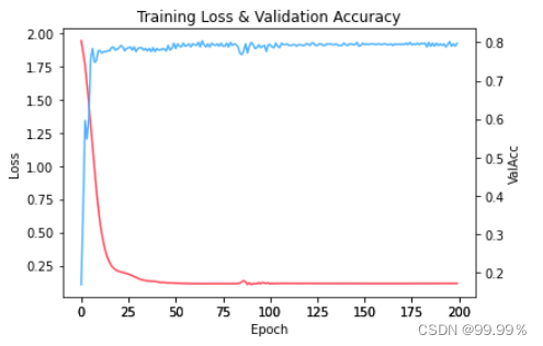
It can be seen that the loss value represented by the red line is getting smaller and smaller as the number of training increases, and the accuracy of the model represented by the blue line is getting higher and higher.
The output obtained from the last layer is subjected to TSNE dimensionality reduction. (TSNE) t-distributed random neighborhood embedding is a nonlinear dimensionality reduction algorithm for exploring high-dimensional data.
It maps multidimensional data to two or more dimensions suitable for human observation.
The classification results are obtained as shown in the figure below:
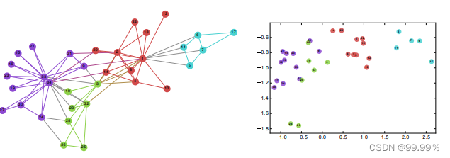
Draw the TSNE dimensionality reduction diagram of the test data:
- from sklearn.manifold import TSNE
- tsne = TSNE()
- out = tsne.fit_transform(test_logits)
- fig = plt.figure()
- for i in range(7):
- indices = test_label == i
- x, y = out[indices].T
- plt.scatter(x, y, label=str(i))
- plt.legend()
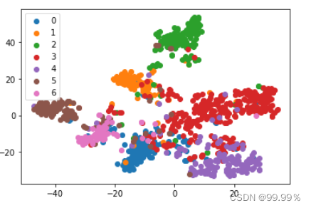
According to the above results: we can successfully divide the collection of papers into 7 distinct categories through the graph convolutional neural network algorithm, which is basically consistent with the original classification of the collection of papers, and the effect is quite impressive.
Category of website: technical article > Blog
Author:cindy
link:http://www.pythonblackhole.com/blog/article/25249/04e82c05ec278ff81d73/
source:python black hole net
Please indicate the source for any form of reprinting. If any infringement is discovered, it will be held legally responsible.
name:
Comment content: (supports up to 255 characters)
no articles